Comparing Endid and Linear DiD

This example illustrates a location-scale treatment effect, where the policy changes both the mean and dispersion of the outcome.

Setup

using Endid
using DataFrames
using Statistics
using Random
using Distributions
using Plots

Random.seed!(42)

N = 80
T_total = 6
tpost1 = 4

unit = repeat(1:N, inner=T_total)
time = repeat(1:T_total, outer=N)
alpha = repeat(randn(N) .* 0.3, inner=T_total)
group = repeat(vcat(fill(1, Int(N / 2)), fill(0, Int(N / 2))), inner=T_total)
post = [t >= tpost1 ? 1 : 0 for t in time]
D = post .* group

epsilon = randn(N * T_total)
y = alpha .+ 0.5 .* D .+ (0.5 .+ 1.0 .* D) .* epsilon

df = DataFrame(unit = unit, time = time, y = y, post_treat = post, group = group)
first(df, 10)

10×5 DataFrame

Row	unit	time	y	post_treat	group
	Int64	Int64	Float64	Int64	Int64
1	1	1	-0.364315	0	1
2	1	2	0.503675	0	1
3	1	3	-0.134998	0	1
4	1	4	1.07253	1	1
5	1	5	1.45887	1	1
6	1	6	-0.688539	1	1
7	2	1	0.79136	0	1
8	2	2	0.540012	0	1
9	2	3	-0.271174	0	1
10	2	4	-0.526821	1	1

Estimation

fit_endid = endid(df, :y, :unit, :time, :post_treat;
                  dvar=:group, num_epochs=10, nboot=1, seed=42)

println(fit_endid)


Training Engression...  20%|█████▋                      |  ETA: 0:01:33
Training Engression... 100%|████████████████████████████| Time: 0:00:23
Running Parallel Bootstrap (n=1)...
Endid Result (common_timing design)
------------------------------
ATT Estimate: -0.068
Std. Error  : NaN
95% CI      : (-0.068, -0.068)

Quantile Treatment Effects (QTE):
9×3 DataFrame
 Row │ quantile  effect      se
     │ Float64   Float64     Float64
─────┼───────────────────────────────
   1 │      0.1  -0.0677664      NaN
   2 │      0.2  -0.0719812      NaN
   3 │      0.3  -0.0700946      NaN
   4 │      0.4  -0.068942       NaN
   5 │      0.5  -0.0724057      NaN
   6 │      0.6  -0.0728971      NaN
   7 │      0.7  -0.0754968      NaN
   8 │      0.8  -0.0692544      NaN
   9 │      0.9  -0.0737824      NaN

Quantile Treatment Effects

p = plot(fit_endid)
savefig(p, "endid_qte.svg")
nothing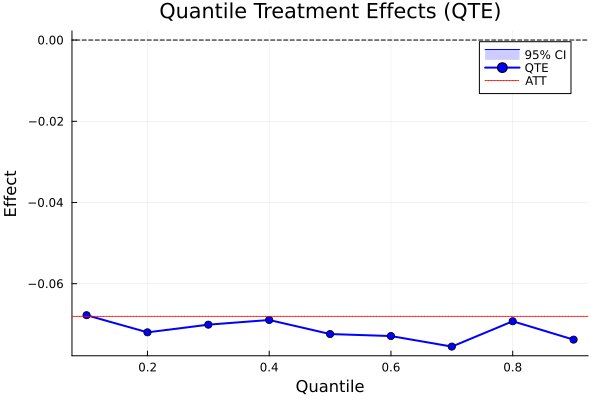

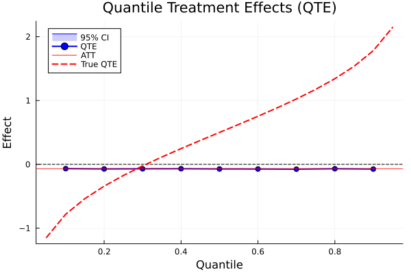
Overlay the analytical QTE, 0.5 + Φ^{-1}(τ):

taus = 0.05:0.05:0.95
true_qte = 0.5 .+ quantile.(Normal(0, 1), taus)

p2 = plot(fit_endid)
plot!(p2, taus, true_qte, label="True QTE", linestyle=:dash, color=:red, linewidth=2)
savefig(p2, "endid_qte_true.svg")
nothing