Getting Started
This vignette uses the matrix API. Rows of Y are units, columns are time periods, controls come first, and treated units come last.
using MSC
using Statistics

sim = simulate_msc(
    ncontrols = 30,
    ntreated = 6,
    T0 = 60,
    T1 = 8,
    tau = 1.5,
    noise = 0.03,
    seed = 11,
)

est = msc_estimate(
    sim.Y,
    sim.N0,
    sim.T0;
    nlambda = 10,
    nfolds = 5,
    max_iter = 1000,
    tol = 1e-6,
)

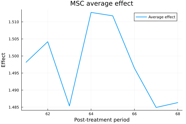
round(est.estimate, digits = 3)1.497effect_matrix returns post-treatment effects by period and treated unit. The ATT is the average of this matrix.
effects = effect_matrix(est)
(
    size = size(effects),
    att = round(mean(effects), digits = 3),
    by_unit = round.(unit_effects(est), digits = 3),
)
(size = (8, 6), att = 1.497, by_unit = [1.515, 1.49, 1.496, 1.484, 1.491, 1.508])The fitted weight matrix is sparse by construction:
first(weights_table(est; atol = 1e-8), 8)8×3 DataFrame
| Row | control | treated | weight |
|---|---|---|---|
| Any | Any | Float64 | |
| 1 | control_6 | treated_1 | -0.094151 |
| 2 | control_16 | treated_1 | -0.111713 |
| 3 | control_20 | treated_1 | 0.0118709 |
| 4 | control_21 | treated_1 | 0.132049 |
| 5 | control_30 | treated_1 | -0.316197 |
| 6 | control_3 | treated_2 | -0.0335523 |
| 7 | control_6 | treated_2 | -0.0631858 |
| 8 | control_20 | treated_2 | 0.0863237 |
Plotting recipes are available when Plots is loaded:
using Plots

plt = plot(
    est;
    title = "MSC average effect",
    xlabel = "Post-treatment period",
    ylabel = "Effect",
)