Illustrative TV-HTE event study (with feedback decomposition) • tvhte

This vignette walks end-to-end through the tvhte API on a synthetic panel that mimics what an applied event-study dataset might look like — persistent outcomes, unit-level heterogeneity in dynamic responses, staggered adoption, and a policy-reactive covariate that adjusts in response to past outcomes. We fit the structural TV-HTE model (Botosaru and Liu 2025), the homogeneous feedback model (Botosaru and Liu 2026), and use both to decompose dynamic event-study responses into direct vs indirect components.

The DGP here is synthetic only because the BL 2025 county-unemployment analysis (their Section 6) does not ship replication data. The workflow on real panel data is identical: swap the simulated Y, Y0, X, X0, t0 for your own panel arranged the same way.

Setup and DGP

library(tvhte)
set.seed(11)

# Mixed cohort: half treated at t = 3, a quarter at t = 5, a quarter never.
N <- 1500; T <- 7
cohorts <- sample(c(3, 5, Inf), N, replace = TRUE, prob = c(0.5, 0.25, 0.25))

sim <- simulate_tvhte(
  N = N, T = T, t0 = cohorts, J = 3,
  rho_Y     = 0.45,   # persistent outcome
  rho_delta = 0.55,   # treatment effect decays with event time
  sigma_U   = 1, sigma_eps = 0.3,
  mu_alpha  = 0,      mu_delta0 = 1.5,    # average DATT at impact = 1.5
  sigma_alpha = 0.6,  sigma_delta0 = 0.5, # heterogeneity in both
  cor_alpha_delta = 0.3,
  beta = 0.4,
  feedback_gamma = c(intercept = 0.1, gamma_Y = 0.25,
                     gamma_X = 0.4,  sigma_eta = 0.3),
  seed = 11
)
str(sim, max.level = 1)
#> List of 9
#>  $ Y     : num [1:1500, 1:7] -1.13 1.688 0.535 1.409 0.081 ...
#>  $ Y0    : num [1:1500] -0.988 -0.272 0.525 0.371 0.689 ...
#>  $ X     : num [1:1500, 1:7, 1] -0.861 -0.735 1.443 -0.617 0.74 ...
#>  $ X0    : num [1:1500] -1.613 -2.34 2.151 -1.091 0.203 ...
#>  $ t0    : num [1:1500] 3 3 Inf 3 3 ...
#>  $ J     : num 3
#>  $ lambda: num [1:1500, 1:2] -0.355 0.016 -0.91 -0.818 0.707 ...
#>  $ delta : num [1:1500, 1:4] 1.571 0.988 2.142 1.116 2.218 ...
#>  $ params:List of 11

The simulated panel has N = 1500 units observed at t = 0, 1, ..., 7. Three cohorts (treated at 3, treated at 5, never treated) are mixed in known proportions. The covariate X_{it} adjusts each period in response to lagged Y and lagged X — the homogeneous-feedback DGP of BL 2026.

Fit the structural model

fit <- tvhte(
  Y  = sim$Y,
  Y0 = sim$Y0,
  t0 = sim$t0,
  J  = sim$J,
  X  = sim$X,
  compute_se = TRUE
)
print(fit)
#> Time-Varying Heterogeneous Treatment Effects (Botosaru-Liu 2025)
#>   N = 1500 units; T = 7 periods; staggered (3 cohorts: 3:n=750, 5:n=381, Inf:n=369); J = 3
#>   log-likelihood = -16054.263   convergence = 0
#> 
#> Common parameters (theta):
#>   rho_Y      = 0.4769   (SE 0.01485)
#>   rho_delta  = 0.5434   (SE 0.01977)
#>   sigma_U    = 1.003
#>   sigma_eps  = 0.1411
#> Prior on lambda_i = (alpha, delta_0):
#>   mu = (0.0125, 1.476)
#>   sd = (0.5972, 0.493),  cor = 0.2837
#> 
#> Covariate coefficients (beta):
#>   beta[1] = 0.3538   (SE 0.02851)
#> 
#> Mean posterior event-time effects (across units):
#>   delta_0 = 1.4757   delta_1 = 0.8021   delta_2 = 0.4357   delta_3 = 0.2371

The QMLE recovers the dynamic parameters cleanly: rho_Y, rho_delta, the covariate coefficient beta, and the prior moments of the correlated random coefficients (alpha_i, delta_{i0}). The “mean posterior event-time effects” line shows the average across units of the unit-level empirical-Bayes trajectories — this is what an event- study plot would show aggregated across units.

Unit-level posterior trajectories

The empirical-Bayes step gives a per-unit (alpha_hat, delta0_hat) plus the full event-time path delta_{i,j} for j = 0..J.

library(graphics)
# Show 30 randomly-chosen treated units' posterior trajectories
treated_idx <- which(is.finite(sim$t0))
sub <- sample(treated_idx, 30)
matplot(0:fit$J, t(fit$delta_path[sub, ]),
        type = "l", col = adjustcolor("grey40", 0.4), lty = 1,
        xlab = "Event time j",
        ylab = "Posterior mean delta_{i,j}",
        main = "Unit-level event-time trajectories (30 random treated units)")
# Overlay the cross-unit mean
lines(0:fit$J, colMeans(fit$delta_path[treated_idx, ]),
      lwd = 2, col = "firebrick")
legend("topright", legend = c("unit-level posteriors", "average"),
       col = c("grey40", "firebrick"), lty = 1, lwd = c(1, 2), bty = "n")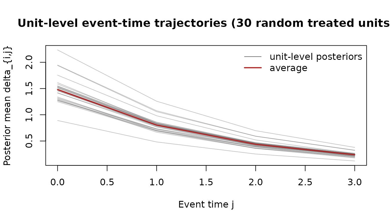

The trajectories fan out because the random coefficient delta_{i0} varies across units. The average path (red) decays at roughly the estimated rho_delta.

Fit the feedback model

fb <- fit_feedback(sim$Y, sim$Y0, sim$X, sim$X0)
print(fb)
#> Homogeneous covariate-feedback process (Botosaru-Liu 2026)
#>   X_it = 0.09722 + 0.2519 * Y_{i,t-1} + 0.3986 * X_{i,t-1} + eta_it
#>   sigma_eta = 0.3008

The covariate X_{it} is modelled as an AR(1) with one lag of Y — the simplest “homogeneous feedback” specification. Coefficients should sit near the true c(0.1, 0.25, 0.4).

Under the BL 2026 factorisation, the structural piece (fit by tvhte()) and the feedback piece (fit by fit_feedback()) are estimated separately — neither needs a parametric specification of the other.

Counterfactual decomposition

simulate_counterfactual() implements BL 2026’s Algorithm 1: it draws latent types from the estimated prior, evolves event-time effects via the AR(1), and propagates (Y, X) jointly using the estimated feedback process. The output is a joint counterfactual path (Y_i^{T,*}, X_i^{T,*}), separating the direct effect (through delta_{i,j}) from the indirect effect (through X_t * beta).

# Counterfactual 1: same units, treatment shifted earlier (t0 = 2)
cf_early <- simulate_counterfactual(fit, fb, t0_star = 2,
                                    N_star = 500, seed = 99)
# Counterfactual 2: same units, never treated
cf_never <- simulate_counterfactual(fit, fb, t0_star = Inf,
                                    N_star = 500, seed = 99)

# Difference at each calendar period gives the total dynamic response.
total_effect <- colMeans(cf_early$Y) - colMeans(cf_never$Y)

# Direct-only counterfactual: same treatment but freeze X at its baseline
# value (no feedback adjustment). We re-build by setting feedback gammas
# that ignore Y_lag and X_lag (so X stays at its intercept + noise).
fb_frozen <- fb
fb_frozen$coef["gamma_Y"] <- 0
fb_frozen$coef["gamma_X"] <- 0
cf_early_direct <- simulate_counterfactual(fit, fb_frozen, t0_star = 2,
                                           N_star = 500, seed = 99)
cf_never_direct <- simulate_counterfactual(fit, fb_frozen, t0_star = Inf,
                                           N_star = 500, seed = 99)
direct_effect <- colMeans(cf_early_direct$Y) - colMeans(cf_never_direct$Y)
indirect_effect <- total_effect - direct_effect

decomp <- data.frame(
  t = 1:T,
  total    = round(total_effect,    3),
  direct   = round(direct_effect,   3),
  indirect = round(indirect_effect, 3)
)
print(decomp)
#>   t total direct indirect
#> 1 1 0.000  0.000    0.000
#> 2 2 1.491  1.491    0.000
#> 3 3 1.658  1.525    0.133
#> 4 4 1.429  1.165    0.264
#> 5 5 1.136  0.803    0.333
#> 6 6 0.726  0.383    0.343
#> 7 7 0.484  0.183    0.301

matplot(decomp$t, decomp[, -1],
        type = "l", lty = c(1, 2, 3), col = c("black", "firebrick", "steelblue"),
        lwd = 2, xlab = "Calendar time", ylab = "Effect on Y",
        main = "Dynamic decomposition: total vs direct + indirect")
abline(h = 0, lty = 3, col = "grey50")
legend("topleft", legend = c("Total", "Direct (delta)", "Indirect (X feedback)"),
       lty = c(1, 2, 3), col = c("black", "firebrick", "steelblue"),
       lwd = 2, bty = "n")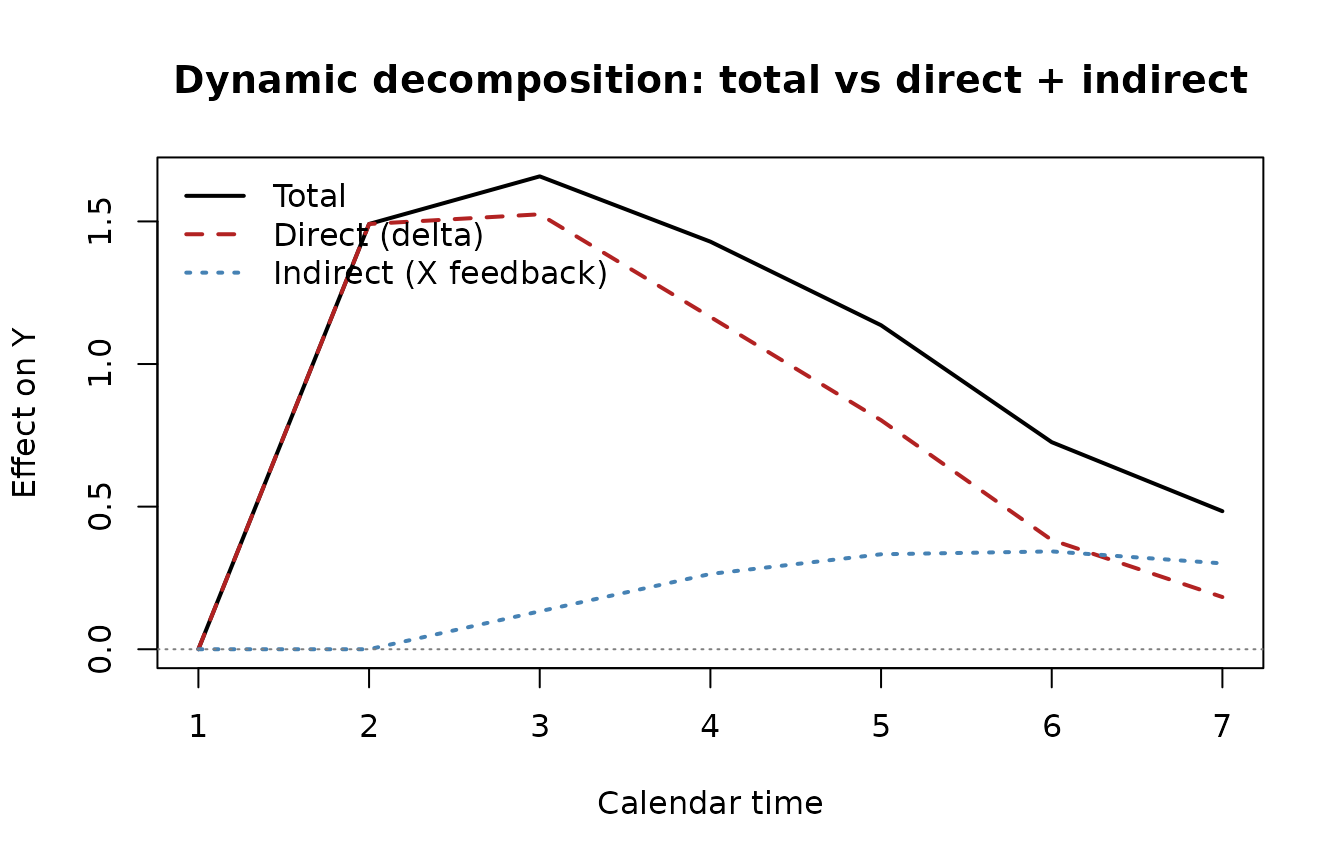

The total dynamic response (black) is the sum of the direct structural effect (red dashed — what the unit would experience holding the covariate path fixed) and the indirect adjustment effect (blue dotted — how much of the response is mediated by the covariate responding to past outcomes and treatment). In the BL 2026 minimum-wage example, the direct effect is the wage response holding firm input demand fixed; the indirect effect is the additional response that flows through firms re-optimising hours and employment composition.

On real data

For an applied dataset, the workflow is the same:

Arrange your panel as (N x T) outcome matrix Y, baseline vector Y0, optional (N x T x K) covariate array X, baseline X0, and length-N treatment-cohort vector t0 (use Inf for never-treated units).
Call tvhte(Y, Y0, t0, J, X) for the structural fit.
Call fit_feedback(Y, Y0, X, X0) for the feedback fit.
Counterfactual decomposition with simulate_counterfactual().

The QMLE step under the Gaussian working prior is consistent for the common parameters even when the true prior on (alpha_i, delta_{i0}) is non-Gaussian (Botosaru and Liu 2025); the empirical-Bayes step achieves ratio optimality. The homogeneous-feedback factorisation delivers separately-identified direct and indirect effects (Botosaru and Liu 2026).

References

Botosaru, Irene and Laura Liu (2025). “Time-Varying Heterogeneous Treatment Effects in Event Studies.” arXiv:2509.13698.
Botosaru, Irene and Laura Liu (2026). “Event Studies with Feedback.” AEA Papers and Proceedings 116: 70–74.