Getting Started

This vignette fits Time-Aware Synthetic Control on simulated panel data. Rows are units and columns are time periods. By default, row 1 is the treated unit and rows 2:N are donors.

using TASC
using Statistics
using Random

Random.seed!(11)

Y, true_params, signal = simulate_tasc(N = 20, T = 80, d = 3, seed = 11)
T0 = 50

model = fit_tasc(
    Y;
    d = 3,
    T0 = T0,
    n_em = 30,
    tol = 1e-4,
)

pred = predict_counterfactual(model, Y)

post = (T0 + 1):size(Y, 2)
att = mean(pred.effect[post])
rmse = sqrt(mean((pred.target[post] .- signal[1, post]) .^ 2))

(att = round(att, digits = 3), rmse = round(rmse, digits = 3))

(att = 0.023, rmse = 0.114)

The returned prediction stores the counterfactual path, treatment-effect path, donor fitted values, and the smoothed state distribution:

keys(pred)

(:target, :donors, :variance, :effect, :state_mean, :state_covariance)

The model-based pointwise interval used in the TASC paper comes from the smoothed latent covariance:

se = sqrt.(max.(pred.variance, 0.0))
lower = pred.target .- 1.96 .* se
upper = pred.target .+ 1.96 .* se

round.((lower[end], pred.target[end], upper[end]), digits = 3)

(-0.128, 0.084, 0.295)

To use the plotting recipe, load Plots and pass the wrapper returned by tasc_plot:

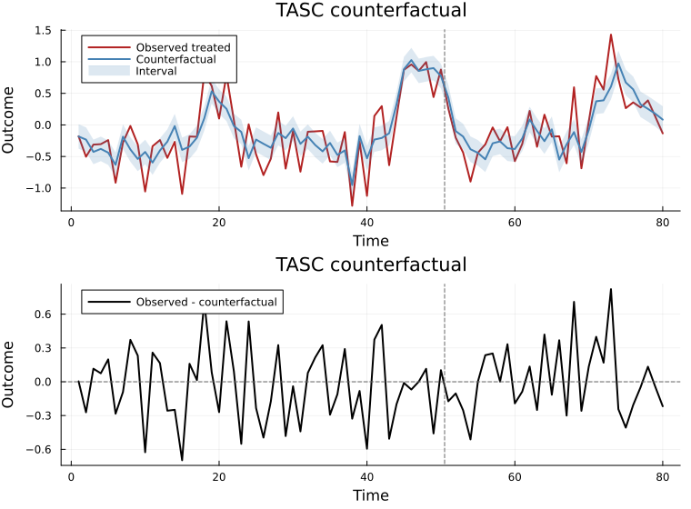
using Plots

plt = plot(
    tasc_plot(model, Y);
    ci = true,
    show_effect = true,
    title = "TASC counterfactual",
    xlabel = "Time",
    ylabel = "Outcome",
)