Introduction to SynthDiD.jl
SynthDiD.jl implements three related estimators for policy evaluation with panel data:
- Synthetic Diff-in-Diff (SDiD) optimizes both unit weights
ωand time weightsλ - Synthetic Control (SC) optimizes unit weights only
- Diff-in-Diff (DiD) uses uniform weights across controls and pre-treatment periods
This tutorial uses the California Proposition 99 tobacco-tax example bundled with the package.
Setup
using SynthDiD
using Plots
using DataFrames
using Random
using Printf

Random.seed!(12345)Random.TaskLocalRNG()California Proposition 99
Load the long-format panel and inspect the first few rows:
df = california_prop99()
first(df, 5)
5×4 DataFrame
| Row | State | Year | PacksPerCapita | treated |
|---|---|---|---|---|
| String15 | Int64 | Float64 | Int64 | |
| 1 | Alabama | 1970 | 89.8 | 0 |
| 2 | Arkansas | 1970 | 100.3 | 0 |
| 3 | Colorado | 1970 | 124.8 | 0 |
| 4 | Connecticut | 1970 | 120.0 | 0 |
| 5 | Delaware | 1970 | 155.0 | 0 |
Convert the panel to the matrix representation expected by the estimators:
setup = panel_matrices(df, :State, :Year, :PacksPerCapita, :treated)
years = collect(setup.times)

println("Y: $(size(setup.Y)), N0 = $(setup.N0), T0 = $(setup.T0)")
Y: (39, 31), N0 = 38, T0 = 19Point Estimates
Estimate all three models on the same treated-control setup:
tau_sdid = synthdid_estimate(setup.Y, setup.N0, setup.T0;
                             units=setup.units, times=years)
tau_sc = sc_estimate(setup.Y, setup.N0, setup.T0;
                     units=setup.units, times=years)
tau_did = did_estimate(setup.Y, setup.N0, setup.T0;
                       units=setup.units, times=years)

println(tau_sdid)
println(tau_sc)
println(tau_did)
Synthetic Diff-in-Diff Estimate
───────────────────────────────────
τ̂ = -15.6038
N₀ = 38, N₁ = 1
T₀ = 19, T₁ = 12
N₀_eff = 16.4, T₀_eff = 2.8
Synthetic Diff-in-Diff Estimate
───────────────────────────────────
τ̂ = -19.6197
N₀ = 38, N₁ = 1
T₀ = 19, T₁ = 12
N₀_eff = 3.8, T₀_eff = 19.0
Synthetic Diff-in-Diff Estimate
───────────────────────────────────
τ̂ = -27.3491
N₀ = 38, N₁ = 1
T₀ = 19, T₁ = 12
N₀_eff = 38.0, T₀_eff = 19.0Compare the resulting treatment effects directly:
println("-" ^ 50)
@printf("%-30s %10s\n", "Estimator", "tau")
println("-" ^ 50)
for (name, est) in [("Diff-in-Diff", tau_did),
                    ("Synthetic Control", tau_sc),
                    ("Synthetic Diff-in-Diff", tau_sdid)]
    @printf("%-30s %10.2f\n", name, est.estimate)
end
println("-" ^ 50)
--------------------------------------------------
Estimator tau
--------------------------------------------------
Diff-in-Diff -27.35
Synthetic Control -19.62
Synthetic Diff-in-Diff -15.60
--------------------------------------------------Standard Errors
With one treated unit, placebo inference is the appropriate variance estimator:
Random.seed!(12345)
se_val = se(tau_sdid; method=:placebo, replications=200)

@printf("Point estimate: %1.2f\n", tau_sdid.estimate)
@printf("Placebo SE:     %1.2f\n", se_val)
@printf("95%% CI:         (%1.2f, %1.2f)\n",
        tau_sdid.estimate - 1.96 * se_val,
        tau_sdid.estimate + 1.96 * se_val)
Point estimate: -15.60
Placebo SE: 9.40
95% CI: (-34.02, 2.81)Plotting
The built-in recipe plots treated and synthetic trajectories together:
p1 = plot(tau_sdid)
savefig(p1, "intro_parallel_trends.svg")
nothing
GKS: cannot open display - headless operation mode active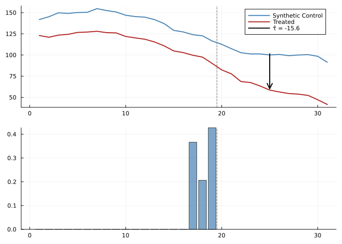
You can also compare all three estimators side by side:
p2 = plot([tau_did, tau_sc, tau_sdid])
savefig(p2, "intro_compare_estimators.svg")
nothing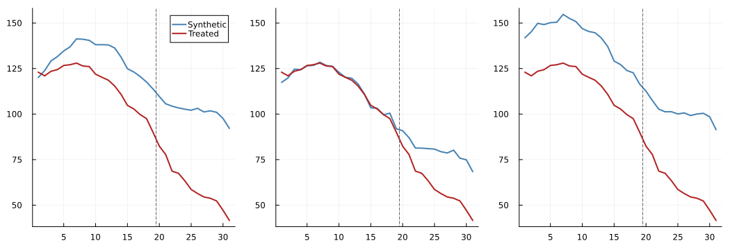
Effect Curves and Weights
Inspect the post-treatment effect path:
curve = effect_curve(tau_sdid)
post_years = years[(setup.T0 + 1):end]

p3 = bar(post_years, curve; label="Per-period effect")
savefig(p3, "intro_effect_curve.svg")
nothing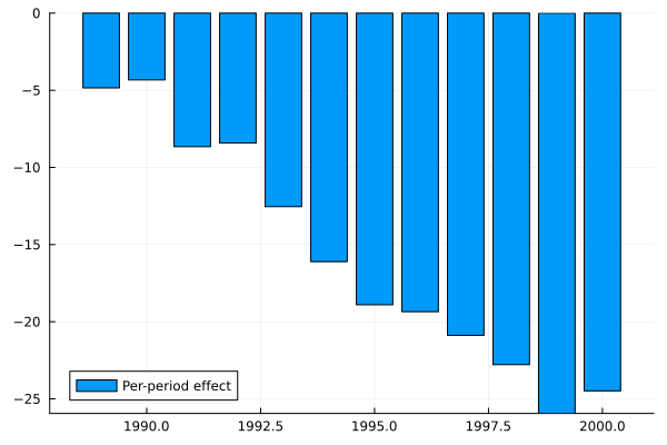
Summarize the most influential control units:
omega = tau_sdid.weights.omega
control_names = setup.units[1:setup.N0]
top_idx = sortperm(omega, rev=true)[1:10]

for i in top_idx
    @printf("%-20s %0.4f\n", control_names[i], omega[i])
end
Nevada 0.1245
New Hampshire 0.1050
Connecticut 0.0783
Delaware 0.0704
Colorado 0.0575
Illinois 0.0534
Nebraska 0.0479
Montana 0.0451
Utah 0.0415
New Mexico 0.0406