More on Plotting

SynthDiD.jl stores unit labels, time labels, and weights alongside each estimate, which makes it straightforward to go beyond the default plot recipe.

Setup

using SynthDiD
using Plots
using DataFrames
using Random

Random.seed!(12345)

Random.TaskLocalRNG()

Real Labels for Units and Time

Pass units and times when estimating so the plots use the original panel labels:

df = california_prop99()
setup = panel_matrices(df, :State, :Year, :PacksPerCapita, :treated)
years = collect(setup.times)

tau_sdid = synthdid_estimate(setup.Y, setup.N0, setup.T0;
                             units=setup.units, times=years)
tau_sc = sc_estimate(setup.Y, setup.N0, setup.T0;
                     units=setup.units, times=years)
tau_did = did_estimate(setup.Y, setup.N0, setup.T0;
                       units=setup.units, times=years)

Synthetic Diff-in-Diff Estimate
───────────────────────────────────
  τ̂  = -27.3491
  N₀ = 38,  N₁ = 1
  T₀ = 19,  T₁ = 12
  N₀_eff = 38.0,  T₀_eff = 19.0

Built-in Plot Recipe

The quickest way to visualize the treatment effect is the package recipe:

p1 = plot(tau_sdid)
savefig(p1, "plotting_recipe.svg")
nothing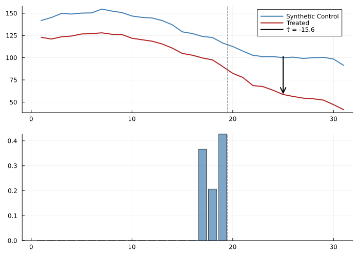

To compare estimators, pass a vector:

p2 = plot([tau_did, tau_sc, tau_sdid])
savefig(p2, "plotting_compare.svg")
nothing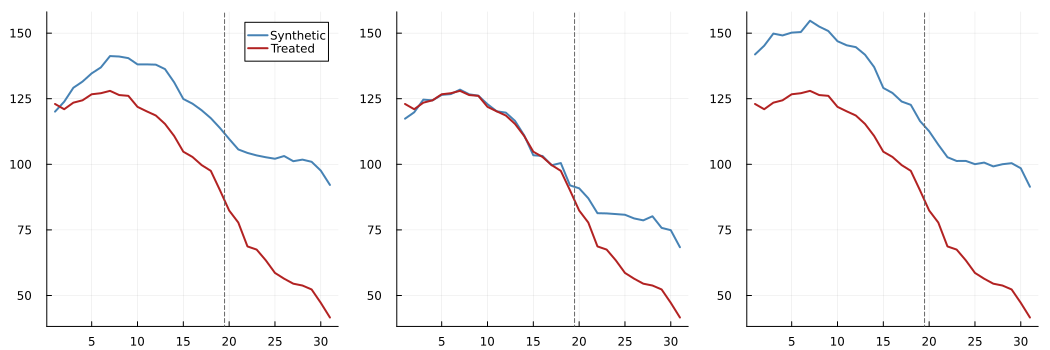

Custom Plot Construction

The estimate object exposes weights and setup, so a custom plot can be built from the saved pieces:

Y = setup.Y
N0 = setup.N0
T0 = setup.T0
omega = tau_sdid.weights.omega

synth = vec(omega' * Y[1:N0, :])
california = vec(Y[N0 + 1, :])

p = plot(years, synth;
    label="Synthetic Control",
    color=:steelblue,
    linewidth=2,
    xlabel="Year",
    ylabel="Packs per Capita")

plot!(p, years, california;
    label="California",
    color=:firebrick,
    linewidth=2)

vline!(p, [years[T0] + 0.5];
    label="",
    color=:gray40,
    linestyle=:dash)
p
savefig(p, "plotting_custom.svg")
nothing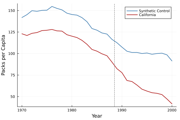

Weight Summaries

The synthdid_controls helper returns the most important unit weights as a DataFrame:

ctrl = synthdid_controls([tau_sdid, tau_sc, tau_did]; mass=0.9)
println(ctrl)

18×4 DataFrame
 Row │ unit            synthdid   synthdid_1  synthdid_2
     │ Any             Float64    Float64     Float64
─────┼───────────────────────────────────────────────────
   1 │ Nevada          0.124489   0.204426     0.0263158
   2 │ New Hampshire   0.105048   0.0453637    0.0263158
   3 │ Connecticut     0.0782873  0.104467     0.0263158
   4 │ Delaware        0.0703681  0.00405026   0.0263158
   5 │ Colorado        0.0575128  0.0133158    0.0263158
   6 │ Illinois        0.0533878  0.0          0.0263158
   7 │ Nebraska        0.0478532  0.0          0.0263158
   8 │ Montana         0.0451352  0.232273     0.0263158
   9 │ Utah            0.0415177  0.396104     0.0263158
  10 │ New Mexico      0.0405683  0.0          0.0263158
  11 │ Minnesota       0.0394946  0.0          0.0263158
  12 │ Wisconsin       0.0366671  0.0          0.0263158
  13 │ West Virginia   0.0335691  0.0          0.0263158
  14 │ North Carolina  0.0328052  0.0          0.0263158
  15 │ Idaho           0.0314682  0.0          0.0263158
  16 │ Ohio            0.0314608  0.0          0.0263158
  17 │ Maine           0.028211   0.0          0.0263158
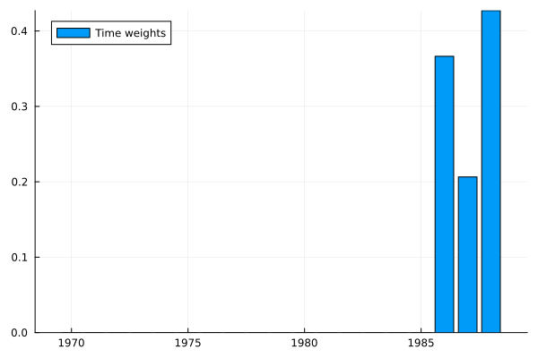
  18 │ Iowa            0.0259386  0.0          0.0263158

You can also inspect time weights directly:

lambda = tau_sdid.weights.lambda
p3 = bar(years[1:T0], lambda; label="Time weights")
savefig(p3, "plotting_time_weights.svg")
nothing