Paper Results
This tutorial reproduces the package's main Proposition 99 estimates and a simple placebo exercise in the style of the original Synthetic Difference-in-Differences paper.
Setup
using SynthDiD
using Plots
using DataFrames
using Statistics
using Random
using Printf

Random.seed!(12345)Random.TaskLocalRNG()California Proposition 99 Application
Estimate the three models on the bundled panel:
df = california_prop99()
setup = panel_matrices(df, :State, :Year, :PacksPerCapita, :treated)
years = collect(setup.times)

tau_sdid = synthdid_estimate(setup.Y, setup.N0, setup.T0;
                             units=setup.units, times=years)
tau_sc = sc_estimate(setup.Y, setup.N0, setup.T0;
                     units=setup.units, times=years)
tau_did = did_estimate(setup.Y, setup.N0, setup.T0;
                       units=setup.units, times=years)

estimates = [tau_did, tau_sc, tau_sdid]
est_names = ["DiD", "SC", "SDiD"]
3-element Vector{String}:
"DiD"
"SC"
"SDiD"Summarize point estimates and placebo standard errors:
point_est = [e.estimate for e in estimates]

Random.seed!(12345)
se_placebo = [se(e; method=:placebo, replications=200) for e in estimates]

println("\n" * "=" ^ 60)
@printf("%-20s %12s %12s\n", "Estimator", "tau", "Placebo SE")
println("=" ^ 60)
for (name, est, se_val) in zip(est_names, point_est, se_placebo)
    @printf("%-20s %12.2f %12.2f\n", name, est, se_val)
end
println("=" ^ 60)
============================================================
Estimator                     tau   Placebo SE
============================================================
DiD                        -27.35         9.22
SC                         -19.62        10.78
SDiD                       -15.60        10.76
============================================================
Plot the three fitted paths together:
p1 = plot(estimates; size=(1000, 350))
savefig(p1, "paper_estimates.svg")
nothing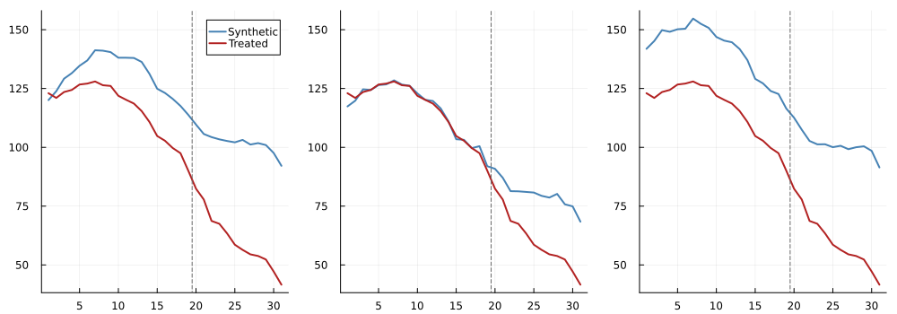
Inspect the largest control and time weights:
unit_weights = synthdid_controls(estimates; weight_type="omega", mass=0.95)
time_weights = synthdid_controls(estimates; weight_type="lambda", mass=0.95)

println(unit_weights)
println(time_weights)
37×4 DataFrame
Row │ unit synthdid synthdid_1 synthdid_2
│ Any Float64 Float64 Float64
─────┼───────────────────────────────────────────────────
1 │ Alabama 0.0263158 0.0 0.0
2 │ Arkansas 0.0263158 0.0 0.00344183
3 │ Colorado 0.0263158 0.0133158 0.0575128
4 │ Connecticut 0.0263158 0.104467 0.0782873
5 │ Delaware 0.0263158 0.00405026 0.0703681
6 │ Georgia 0.0263158 0.0 0.00158841
7 │ Idaho 0.0263158 0.0 0.0314682
8 │ Illinois 0.0263158 0.0 0.0533878
9 │ Indiana 0.0263158 0.0 0.0101355
10 │ Iowa 0.0263158 0.0 0.0259386
11 │ Kansas 0.0263158 0.0 0.0216052
12 │ Kentucky 0.0263158 0.0 0.0
13 │ Louisiana 0.0263158 0.0 0.0
14 │ Maine 0.0263158 0.0 0.028211
15 │ Minnesota 0.0263158 0.0 0.0394946
16 │ Mississippi 0.0263158 0.0 0.0
17 │ Missouri 0.0263158 0.0 0.0078025
18 │ Montana 0.0263158 0.232273 0.0451352
19 │ Nebraska 0.0263158 0.0 0.0478532
20 │ Nevada 0.0263158 0.204426 0.124489
21 │ New Hampshire 0.0263158 0.0453637 0.105048
22 │ New Mexico 0.0263158 0.0 0.0405683
23 │ North Carolina 0.0263158 0.0 0.0328052
24 │ North Dakota 0.0263158 0.0 0.0
25 │ Ohio 0.0263158 0.0 0.0314608
26 │ Oklahoma 0.0263158 0.0 0.0
27 │ Pennsylvania 0.0263158 0.0 0.0153521
28 │ Rhode Island 0.0263158 0.0 0.00104159
29 │ South Carolina 0.0263158 0.0 0.0
30 │ South Dakota 0.0263158 0.0 0.00408709
31 │ Tennessee 0.0263158 0.0 0.0
32 │ Texas 0.0263158 0.0 0.00977753
33 │ Utah 0.0263158 0.396104 0.0415177
34 │ Vermont 0.0263158 0.0 0.0
35 │ Virginia 0.0263158 0.0 0.0
36 │ West Virginia 0.0263158 0.0 0.0335691
37 │ Wisconsin 0.0263158 0.0 0.0366671
19×4 DataFrame
Row │ unit synthdid synthdid_1 synthdid_2
│ Any Float64 Float64 Float64
─────┼─────────────────────────────────────────
1 │ 1970 0.0526316 0.0 0.0
2 │ 1971 0.0526316 0.0 0.0
3 │ 1972 0.0526316 0.0 0.0
4 │ 1973 0.0526316 0.0 0.0
5 │ 1974 0.0526316 0.0 0.0
6 │ 1975 0.0526316 0.0 0.0
7 │ 1976 0.0526316 0.0 0.0
8 │ 1977 0.0526316 0.0 0.0
9 │ 1978 0.0526316 0.0 0.0
10 │ 1979 0.0526316 0.0 0.0
11 │ 1980 0.0526316 0.0 0.0
12 │ 1981 0.0526316 0.0 0.0
13 │ 1982 0.0526316 0.0 0.0
14 │ 1983 0.0526316 0.0 0.0
15 │ 1984 0.0526316 0.0 0.0
16 │ 1985 0.0526316 0.0 0.0
17 │ 1986 0.0526316 0.0 0.366471
18 │ 1987 0.0526316 0.0 0.206453
19 │ 1988 0.0526316 0.0 0.427076Placebo Simulations
A basic placebo routine can be used to summarize how noisy the estimator is under resampling from the donor pool:
function run_placebo_sims(Y, N0, T0; n_sims=100)
    N1 = size(Y, 1) - N0
    estimates = Float64[]

    for sim in 1:n_sims
        ind = rand(1:N0, N0)
        n0_new = length(ind) - N1
        if n0_new < 1
            continue
        end

        try
            est = synthdid_estimate(Y[ind, :], n0_new, T0)
            push!(estimates, est.estimate)
        catch
            continue
        end
    end

    estimates
end

Random.seed!(12345)
placebo_est = run_placebo_sims(setup.Y, setup.N0, setup.T0; n_sims=100)
100-element Vector{Float64}:
7.832393613101248
11.793009338278019
2.4936747159261383
3.6162466871739127
-30.45277955324606
-31.414605681253725
-0.1311947464243186
1.6836535192820818
-33.18444781165256
-3.115958244269219
⋮
-2.2152859724945806
9.481391330878104
2.7368014255362976
-9.401734430927615
2.8407309878174196
7.090025282303433
-13.1803013747466
8.942570173030507
17.729722244216696Summarize and visualize the placebo distribution:
@printf("Mean: %1.2f\n", mean(placebo_est))
@printf("Std:  %1.2f\n", std(placebo_est))
@printf("RMSE: %1.2f\n", sqrt(mean(placebo_est .^ 2)))
Mean: -1.54
Std: 9.24
RMSE: 9.32p2 = histogram(placebo_est;
bins=20,
label="Placebo estimates",
xlabel="Estimated treatment effect",
ylabel="Frequency",
title="Placebo Simulation (100 replications)",
color=:steelblue,
alpha=0.7)
vline!([tau_sdid.estimate];
label="SDiD estimate",
color=:firebrick,
linewidth=2)
savefig(p2, "paper_placebo_histogram.svg")
nothing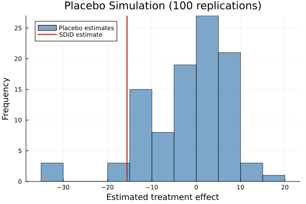
Interpretation
Across these examples, SDiD produces a more conservative estimate than synthetic control and a much smaller effect than plain DiD, reflecting the balance obtained by jointly choosing unit and time weights.