---
code-fold: true
---
# Interpreting OLS: Outcome Weights
```{r}
#| include: false
teal <- "#0E6473"; rust <- "#9E4318"
vtab <- function(x, d = 3) knitr::kable(data.frame(value = round(x, d)), col.names = "value")
mtab <- function(x, d = 3) knitr::kable(round(x, d))
```
The companion chapter [Interpreting OLS: Effect Weights](interpreting-ols.qmd) treats the OLS coefficient as a weighted average of unobserved effects and asks whose effect $\hat\beta$ estimates. We can read the same Frisch--Waugh--Lovell identity as a weighting of observed outcomes. This second reading asks which rows move $\hat\beta$ and in which direction. Both sets of weights can be calculated in OLS, but only here is the thing being weighted also observed: every contribution $\omega_i y_i$ is in the data. The outcome representation also extends beyond OLS.
## The other reading of FWL
Residualise the regressor of interest $V$ on the controls $X$, write $\tilde V_i$ for the residual, and recall the residual-on-residual form of the coefficient, @eq-fwl:
$$ \hat\beta = \frac{\sum_{i=1}^n \tilde V_i y_i}{\sum_{i=1}^n \tilde V_i^2}. $$ {#eq-outcome-weights-1}
The previous chapter groups $\tilde V_i$ with $V_i$ and writes $\hat\beta$ as a weighting $w_i=\tilde V_iV_i$ of effects (@eq-weff). If we instead group each residual with its outcome $y_i$, the same expression becomes a linear combination of the observed outcomes:
$$ \hat\beta = \sum_{i=1}^n \omega_i y_i, \qquad \omega_i = \frac{\tilde V_i}{\sum_{j=1}^n \tilde V_j^2}. $$ {#eq-omega}
@eq-omega is the same algebra rearranged, but a different object from the effect weights.
| | Weights on outcomes $\omega_i$ | Weights on effects $w_i$ |
|---|---|---|
| Weights what | the observed $y_i$ | that observation's own effect $\beta_i$ |
| Sign | signed, sums to zero | can be signed; non-negative for binary $D$ with saturated controls |
| Computable | weight and weighted outcome | weight yes; weighted effect no, because $\beta_i$ is unseen |
| Holds when | always, it is algebra | as a causal average when the error remainder vanishes |
| Answers | which rows drive $\hat\beta$, any wrong sign | is this the effect I meant, whose effect |
Two constraints pin $\omega_i$ down, both from @eq-omega. An intercept among the controls makes $\sum_i \tilde V_i = 0$, so the weights **sum to zero**. And $\sum_i \tilde V_i V_i = \sum_i \tilde V_i^2$ makes the weighted regressor **sum to one**, $\sum_i \omega_i V_i = 1$.
Use this reading when overlap is in doubt and a row may enter with the wrong sign. For binary treatment, the effect weight $w_i=(D_i-\hat D_i)D_i$ can flag a treated row with $\hat D_i>1$, but every control has effect weight zero; the outcome weights expose both sides of the realised comparison. Keep the effect reading for questions about the estimand.
## What the outcome weights look like
Take the simple regression of $y$ on $x$ with an intercept, so $\tilde V_i = x_i - \bar x = d_i$ and
$$ \omega_i = \frac{d_i}{\sum_j d_j^2}. $$ {#eq-outcome-weights-2}
Unlike the leverage weights $d_i^2$ on the observed deviation slopes in the companion chapter — non-negative, growing with the *square* of distance — this is **linear in $d_i$, and so signed**: a point left of $\bar x$ enters $\hat\beta$ with a negative coefficient on its outcome, a point right of it positive. The structural effect weight is instead $d_ix_i$, which need not equal $d_i^2$. The outcome weight is not a slope and does not involve $\bar y$; it is simply a signed weight on the observed $y_i$.
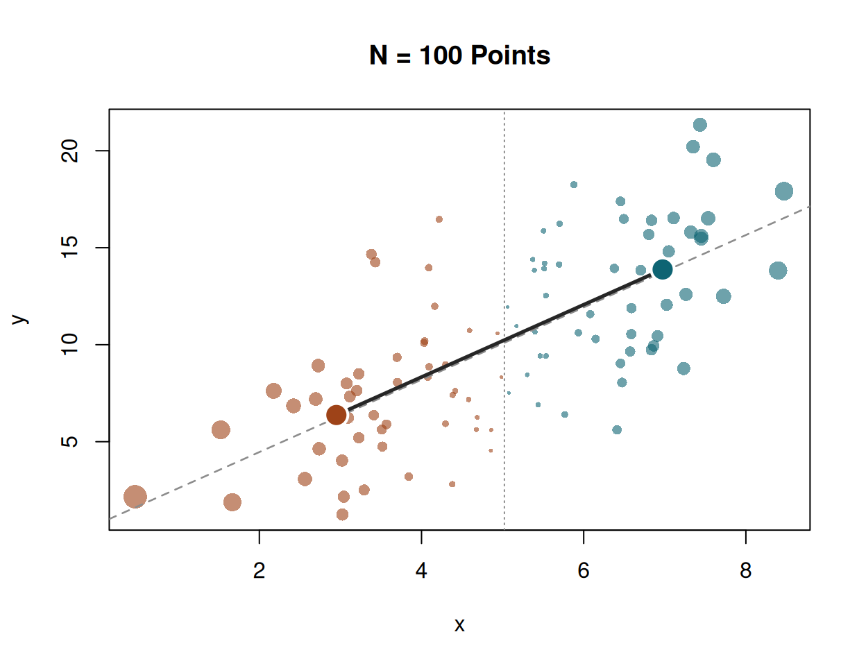
**Simulation — simple regression.** To see it, we simulate $n = 100$ points — regressor $x_i \sim N(5, 2^2)$ and outcome $y_i = 2 x_i + \varepsilon_i$ with $\varepsilon_i \sim N(0, 3^2)$ — then size each point by $|\omega_i|$ and colour it by sign.
```{r}
#| fig-width: 6.5
#| fig-height: 5
#| fig-cap: "Outcome weights in a 100-point sample. Each small point's **size scales with its weight** $|\\omega_i|$, coloured by sign — teal ($\\omega_i > 0$) pushes $\\hat\\beta$ up, rust ($\\omega_i < 0$) pulls it down; the dotted line is the fulcrum $x = \\bar x$. The two large dots are the $|d|$-weighted centroids of the points left and right of $\\bar x$; the solid segment joining them has slope $\\hat\\beta$, and the dashed line is the OLS fit (same slope, shifted through the grand mean)."
set.seed(3)
n <- 100; x <- rnorm(n, 5, 2); y <- 2 * x + rnorm(n, 0, 3)
xb <- mean(x); d <- x - xb; om <- d / sum(d^2); col <- ifelse(om >= 0, teal, rust)
R <- d > 0; L <- d < 0
xR <- sum(abs(d[R]) * x[R]) / sum(abs(d[R])); yR <- sum(abs(d[R]) * y[R]) / sum(abs(d[R]))
xL <- sum(abs(d[L]) * x[L]) / sum(abs(d[L])); yL <- sum(abs(d[L]) * y[L]) / sum(abs(d[L]))
plot(x, y, pch = 16, cex = 0.35 + 2 * abs(om) / max(abs(om)),
     col = paste0(col, "99"), xlab = "x", ylab = "y", main = "N = 100 Points")
abline(v = xb, lty = 3, col = "grey55")
abline(lm(y ~ x), lwd = 1.3, lty = 2, col = "grey55")
segments(xL, yL, xR, yR, lwd = 2.6, col = "grey15")
points(c(xL, xR), c(yL, yR), pch = 21, bg = c(rust, teal), col = "white", cex = 2.3, lwd = 2)
vtab(c(`$\\sum_i \\omega_i$`   = sum(om),      `$\\sum_i \\omega_i x_i$` = sum(om * x),
        `positive mass` = sum(om[om > 0]), `negative mass` = sum(om[om < 0]),
        `OLS`          = coef(lm(y ~ x))[[2]], `$\\sum_i \\omega_i y_i$` = sum(om * y)), 4)
```
The printed sums confirm @eq-omega: the weights split at $\bar x$ into a positive mass ($\approx +0.25$) and an equal negative one ($\approx -0.25$), and $\sum_i \omega_i x_i = 1$.
But the figure shows more. Split the points at $\bar x$, weight each side by $|d_i|$, and take its centroid — the two large dots. **The segment joining them has slope $\hat\beta$:** the OLS slope is the rise over run between the low-$x$ and high-$x$ weighted centres.
The dashed fit shares that slope, shifted through the grand mean, so the two coincide only when the sides balance. This collapse to two points falls out of the slope formula.
### Why it collapses to two points
Write $d_i = x_i - \bar x$. Because $\sum_i d_i = 0$, the positive and negative sides carry equal total weight $W = \sum_{i: d_i > 0} d_i$. An inner product with $d$ is therefore a between-group contrast: for any variable $v$,
$$ d \cdot v = W(\bar v_R - \bar v_L), $$ {#eq-outcome-weights-4}
where $\bar v_R$ and $\bar v_L$ are the $|d_i|$-weighted means on each side of $\bar x$. The slope $\hat\beta = d \cdot y\, /\, d \cdot x$ is the ratio of two such contrasts; $W$ cancels:
$$ \hat\beta = \frac{\bar y_R - \bar y_L}{\bar x_R - \bar x_L}. $$ {#eq-outcome-weights-5}
That is the rise over run between the two $|d|$-weighted centroids — the two dots in the figure.
## When the sign flips
In simple regression the sign of $\omega_i$ is just the side of the mean: half the weights are negative, structurally, and a low-$x$ point *should* count against a high-$x$ one. With controls $\tilde V_i$ becomes a *residual*, and a row can flip to the sign its raw position denies. Outcome weights reveal that realised extrapolation for treated and control rows alike; binary effect weights omit the control rows because $D_i=0$ makes their effect weight zero.
With a binary treatment $D$ and covariate $x$, the weight $\omega_i \propto \tilde V_i = D_i - \hat D_i$, with $\hat D$ the fitted linear projection of $D$ on $(1, x)$. Regressed on $D$ alone, every treated unit is positive and every control negative — the *structural* pattern, producing $\hat\beta = \bar y_1 - \bar y_0$. Add $x$ and the fitted $\hat D_i$ can leave $[0, 1]$, often where treatment and control overlap poorly. A treated unit with $\hat D_i > 1$ gets $\tilde V_i < 0$, so its outcome is subtracted from $\hat\beta$; a control with $\hat D_i<0$ gets $\tilde V_i>0$, so its outcome is added. These are **wrong-sign outcome weights**, evidence that the fitted linear comparison is extrapolating.
Two qualifications keep this diagnostic in its lane. First, out-of-range the other way is not a sign reversal: a treated unit with $\hat D_i<0$ remains positive and a control with $\hat D_i>1$ remains negative. Second, $\hat D_i$ is a sample fitted value. Leaving $[0,1]$ is evidence of realised linear extrapolation, not proof that the population propensity is out of range or that common support literally fails; sampling error and functional-form approximation can also produce it. Conversely, in-range fits do not establish overlap or the conditional mean-independence assumption needed for a design-based causal interpretation. With a continuous regressor there is no bounded range to leave, so leverage rather than sign carries the diagnostic.
A wrong-sign outcome weight means the fitted regression contrast reaches beyond its conventional treated-versus-control comparison, and $\hat\beta$ can leave the convex hull of the observed outcomes. Whether it matters depends on the data — a sensitivity check is one trim away.
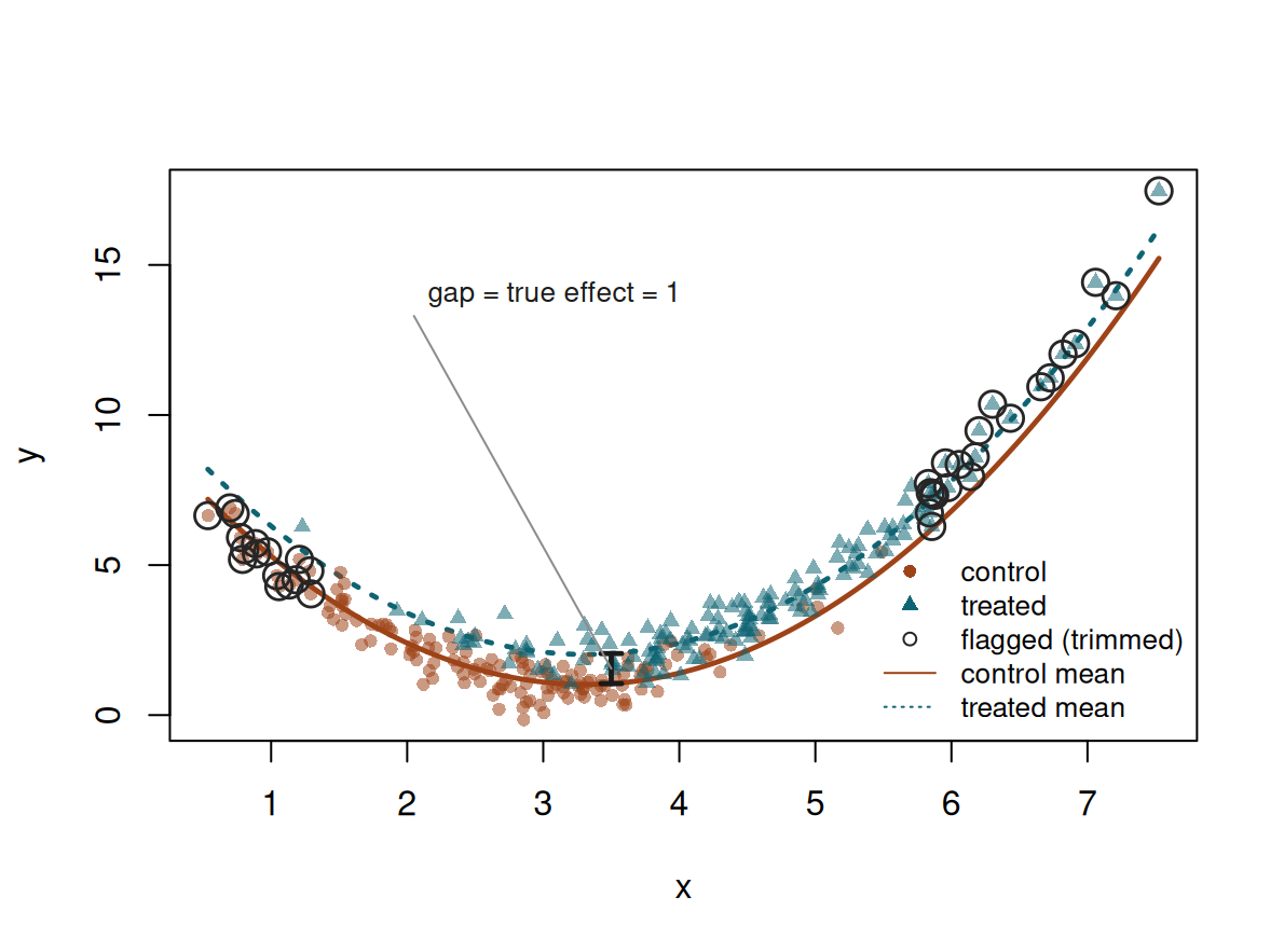
**Simulation — thin overlap on a curved baseline.** The DGP: 150 controls near $x = 2.5$ and 150 treated near $x = 4.5$ (both sd $1.1$), with $y_i = D_i + 0.8\,(x_i - 3.5)^2 + 0.3\,x_i + \varepsilon_i$, $\varepsilon_i \sim N(0, 0.5^2)$ — a constant true effect of $1$ sitting on a convex baseline.
```{r}
#| fig-width: 6.2
#| fig-height: 4.6
#| message: false
#| warning: false
#| fig-cap: "Thin overlap on a convex baseline. The two curves are the true means — control (rust, solid) and treated (teal, dotted), a constant $1$ apart (arrow). Controls sit low on the curve and treated high; the groups share only the middle. Ringed points have wrong-sign outcome weights: treated units with $\\hat D_i>1$ or controls with $\\hat D_i<0$. The straight $y \\sim D + x$ reports $\\hat\\beta = 0.69$; dropping the flagged units, or reweighting to the overlap, restores $\\approx 1$."
set.seed(7)
n <- 150
x <- c(rnorm(n, 2.5, 1.1), rnorm(n, 4.5, 1.1))
d <- c(rep(0, n), rep(1, n))
y <- 1.0 * d + 0.8 * (x - 3.5)^2 + 0.3 * x + rnorm(2 * n, 0, 0.5)
df <- data.frame(y, d, x)
X <- cbind(1, x); dh <- as.vector(X %*% solve(crossprod(X)) %*% t(X) %*% d)
flag <- (d == 1 & dh > 1) | (d == 0 & dh < 0)
pch <- ifelse(d == 1, 17, 16); col <- ifelse(d == 1, teal, rust)
plot(x, y, type = "n", xlab = "x", ylab = "y")
xs <- seq(min(x), max(x), length = 200)
mc <- function(z) 0.8 * (z - 3.5)^2 + 0.3 * z              # true control mean E[y | x, D = 0]
lines(xs, mc(xs),     col = rust, lwd = 2.4)               # control mean
lines(xs, mc(xs) + 1, col = teal, lwd = 2.4, lty = 3)      # treated mean = control + true effect (1)
points(x, y, pch = pch, col = paste0(col, "88"), cex = 0.85)               # all points, by group
points(x[flag], y[flag], pch = 1, col = "grey15", cex = 1.7, lwd = 1.4)    # ring the flagged units
arrows(3.5, mc(3.5), 3.5, mc(3.5) + 1, code = 3, length = 0.05, angle = 90, lwd = 2.4, col = "grey10")
segments(3.5, mc(3.5) + 0.5, 2.05, 13.3, col = "grey55", lwd = 1)
text(2.0, 14, "gap = true effect = 1", pos = 4, cex = 0.82, col = "grey10")
legend("bottomright", bty = "n", cex = 0.82,
       legend = c("control", "treated", "flagged (trimmed)", "control mean", "treated mean"),
       pch = c(16, 17, 1, NA, NA), lty = c(NA, NA, NA, 1, 3),
       col = c(rust, teal, "grey15", rust, teal))
w_ato <- WeightIt::weightit(d ~ x, data = df, method = "glm", estimand = "ATO")
vtab(c(`flagged units`      = sum(flag),
        `$\\hat\\beta$ (full)`        = coef(lm(y ~ d + x))[["d"]],
        `$\\hat\\beta$ (trimmed)`     = coef(lm(y ~ d + x, data = df[!flag, ]))[["d"]],
        `$\\hat\\beta$ (overlap-wtd)` = coef(lm(y ~ d + x, weights = w_ato$weights))[["d"]]), 3)
```
Thirty-seven units carry the wrong sign, all in the non-overlapping tails. Trim them and $\hat\beta$ jumps from $0.69$ to $0.99$; the overlap weights (`"ATO"`, Li, Morgan, and Zaslavsky 2018) give $0.98$. Either fix confirms the estimate leaned on the extrapolation, read off the regression itself with no separate model. Had the outcome been linear, the same trim would barely move $\hat\beta$: the wrong-sign weights are still there, but they are harmless. The check tells you which case you are in.
This is the implied-weights diagnostic of Chattopadhyay and Zubizarreta (2023); their `lmw` package computes the weights and the balance, extrapolation, and influence diagnostics built on them, and `OutcomeWeights` (Knaus 2024) carries it to machine-learning estimators. The mainstream overlap check takes the other route, through the propensity score (`WeightIt` for estimation, `cobalt` for balance, and Crump et al. 2009 for trimming); both routes reach the same conclusion.
## Out of OLS: the same weights beyond the linear model
The outcome reading has one advantage the effect reading lacks: it survives leaving OLS. Any estimator that can be written $\hat\tau = \sum_i \omega_i Y_i = \boldsymbol\omega' \boldsymbol Y$ — a linear combination of the observed outcomes — *has* outcome weights, whatever machinery produced them.
Knaus (2024) makes this the organising idea, and his `OutcomeWeights` package computes $\boldsymbol\omega$ for AIPW, double machine learning, and the causal forest.
### The weights, derived
The OLS outcome weights (@eq-omega) followed from one fact: in the FWL numerator $\sum_i \tilde V_i y_i$, the outcome $y_i$ appears once, linearly, so $\hat\beta = \sum_i \omega_i y_i$ with $\omega_i = \tilde V_i / \sum_j \tilde V_j^2$. The same fact holds whenever the outcome model is a *smoother* — a map $\hat{\boldsymbol m} = \boldsymbol S \boldsymbol Y$ that is linear in the training outcomes. Substituting $\boldsymbol S \boldsymbol Y$ for $\hat{\boldsymbol m}$ keeps $\boldsymbol Y$ linear in the numerator, and reading off its coefficient gives $\boldsymbol\omega$. We carry this out for PLR and AIPW.
*PLR.* Take the partially-linear estimator (the R-learner behind the causal forest). It is FWL with the projections done by a flexible learner: residualise treatment and outcome on the covariates, then regress one residual on the other,
$$ \hat\tau = \frac{\sum_i (D_i - \hat e_i)(Y_i - \hat m_i)}{\sum_i (D_i - \hat e_i)^2}, $$ {#eq-outcome-weights-6}
with $\hat e = \hat E[D \mid X]$ and $\hat m = \hat E[Y \mid X]$ the fitted nuisances.
The outcome nuisance is a *smoother*: its fitted values are a linear map of the training outcomes, $\hat{\boldsymbol m} = \boldsymbol S \boldsymbol Y$ — true for OLS, ridge, kernels, and honest forests alike. The word *honest* carries weight there. If the learner's structure is itself chosen using the outcomes — splits grown on the same $\boldsymbol Y$ being predicted, a lasso whose active set is outcome-selected, boosting — then $\boldsymbol S$ depends on $\boldsymbol Y$ and the map stops being linear in it. What follows then holds *conditional on the fitted learner*, which is the weaker claim: the weights describe the estimate you got rather than a globally linear estimator. Honesty and cross-fitting are what restore the clean reading, by fitting the structure on data other than the outcomes being weighted. So the outcome residual is $\boldsymbol Y - \hat{\boldsymbol m} = (\mathbf I - \boldsymbol S)\boldsymbol Y$. Writing $\tilde{\boldsymbol D} = \boldsymbol D - \hat{\boldsymbol e}$ for the treatment residual and substituting,
$$ \hat\tau = \frac{\tilde{\boldsymbol D}'(\mathbf I - \boldsymbol S)\,\boldsymbol Y}{\tilde{\boldsymbol D}'\tilde{\boldsymbol D}}. $$ {#eq-outcome-weights-7}
Now $\boldsymbol Y$ appears once, linearly, in the numerator. Read off its coefficient and the weights are done:
$$ \hat\tau = \boldsymbol\omega'\boldsymbol Y, \qquad \boldsymbol\omega' = \frac{\tilde{\boldsymbol D}'(\mathbf I - \boldsymbol S)}{\tilde{\boldsymbol D}'\tilde{\boldsymbol D}}. $$ {#eq-omega-ml}
That is @eq-omega — the OLS weights — with the projection annihilator $\boldsymbol M_X$ replaced by the smoother annihilator $\mathbf I - \boldsymbol S$. OLS is the case of a linear learner, $\boldsymbol S = \boldsymbol P_X$: there $\boldsymbol S$ is a projection, $\mathbf I - \boldsymbol S = \boldsymbol M_X$, and @eq-omega-ml is @eq-omega exactly. Component by component, the weight on observation $i$ is
$$ \omega_i = \frac{\tilde D_i - \sum_j S_{ji}\,\tilde D_j}{\sum_k \tilde D_k^2}: $$ {#eq-omega-plr-i}
the treatment residual of unit $i$, minus how much other units' treatment residuals leak to $i$ through the outcome smoother, normalised by the total treatment-residual variance.
The outcome weights tell which rows drive the estimate; the *effect* weights tell whose effect it estimates. Substitute $Y_i = \tau_i D_i + m(X_i) + \varepsilon_i$ into the PLR numerator. With consistent nuisances $\hat m \approx m$, the noise vanishes in expectation and the numerator reduces to $\sum_i \tilde D_i D_i \tau_i$, so the effect weight on $\tau_i$ is $\tilde D_i D_i = (D_i - e_i) D_i$. Since $D$ is binary ($D_i^2 = D_i$),
$$ E[\tilde D_i D_i \mid X_i] = E[D_i \mid X_i] - e_i\, E[D_i \mid X_i] = e_i - e_i^2 = e_i(1 - e_i). $$ {#eq-outcome-weights-8}
The denominator $\tilde{\boldsymbol D}'\tilde{\boldsymbol D} = \sum_i \tilde D_i^2$ has the same expectation, $\sum_i e_i(1 - e_i)$, since $\text{Var}(D_i \mid X_i) = e_i(1 - e_i)$. Both numerator and denominator weight by propensity variance, and the ratio is the variance-weighted average treatment effect,
$$ \tau_{\text{VWATE}} = \frac{\sum_i e(X_i)(1 - e(X_i))\,\tau(X_i)}{\sum_i e(X_i)(1 - e(X_i))}, $$ {#eq-vwate}
not the plain ATE $\bar\tau = n^{-1}\sum_i \tau_i$. The two coincide when effects are constant, or when treatment is randomly assigned so that $e(1-e)$ is the same everywhere. Neither condition is necessary. All that is required is that $\tau(X)$ be uncorrelated with the weight $e(X)(1-e(X))$: heterogeneity that happens not to line up with propensity variance leaves the two equal. The weighting is the same $e(1-e)$ that appeared in the previous chapter's @eq-angrist, where Angrist (1998) showed OLS with saturated strata weights each stratum by $n_x \hat D(x)(1 - \hat D(x))$. That result required discrete strata and saturated controls; @eq-vwate is the same propensity-variance weighting with continuous covariates and a flexible learner. The individual $\tau(X_i)$ are never observed or estimated — they are the structural unit-level effects in $Y_i = \tau(X_i) D_i + m(X_i) + \varepsilon_i$. PLR returns one number, $\hat\tau$, that converges to their $e(1-e)$-weighted average; to estimate $\tau(X_i)$ itself one needs a CATE estimator (a causal forest, say).
Three moves did it: write the estimator, substitute the smoother $\hat{\boldsymbol m} = \boldsymbol S \boldsymbol Y$, read off the coefficient on $\boldsymbol Y$. They work for any estimator built from smoothers; only the operator on $\boldsymbol Y$ changes. AIPW is worth carrying through, because its operator is more than $\mathbf I - \boldsymbol S$.
*AIPW.* With outcome smoothers $\hat{\boldsymbol\mu}_1 = \boldsymbol S_1 \boldsymbol Y$, $\hat{\boldsymbol\mu}_0 = \boldsymbol S_0 \boldsymbol Y$ and propensity $\hat{\boldsymbol e}$, the score of unit $i$ is
$$ \psi_i = \hat\mu_{1i} - \hat\mu_{0i} + \frac{D_i}{\hat e_i}\,(Y_i - \hat\mu_{1i}) - \frac{1 - D_i}{1 - \hat e_i}\,(Y_i - \hat\mu_{0i}), \qquad \hat\tau = \frac1n \sum_i \psi_i. $$ {#eq-outcome-weights-9}
Each $\hat\mu_{ji}$ is $(\boldsymbol S_j \boldsymbol Y)_i$, so $\boldsymbol Y$ again enters only linearly; collecting its coefficient gives $\hat\tau = \boldsymbol\omega' \boldsymbol Y$ with
$$ \boldsymbol T = \boldsymbol S_1 - \boldsymbol S_0 + \operatorname{diag}\!\Big(\tfrac{\boldsymbol D}{\hat{\boldsymbol e}}\Big)(\mathbf I - \boldsymbol S_1) - \operatorname{diag}\!\Big(\tfrac{1 - \boldsymbol D}{1 - \hat{\boldsymbol e}}\Big)(\mathbf I - \boldsymbol S_0), \qquad \boldsymbol\omega' = \frac{\mathbf 1' \boldsymbol T}{n}. $$ {#eq-outcome-weights-10}
That is, $\omega_j$ is the $j$-th column-sum of $\boldsymbol T$ divided by $n$: observation $j$'s outcome enters the ATE through its direct IPW term and through its indirect contribution via the two outcome smoothers $\boldsymbol S_1$, $\boldsymbol S_0$ to every other unit's augmentation correction.
Comparing the two:
| | PLR (@eq-omega-ml) | AIPW |
|---|---|---|
| Matrix form | $\boldsymbol\omega' = \tilde{\boldsymbol D}'(\mathbf I - \boldsymbol S)\,/\,\tilde{\boldsymbol D}'\tilde{\boldsymbol D}$ | $\boldsymbol\omega' = \mathbf 1'\boldsymbol T\,/\,n$ |
| Per unit | $\omega_i = \bigl(\tilde D_i - \sum_j S_{ji}\tilde D_j\bigr)\,/\,\sum_k \tilde D_k^2$ | $\omega_j = \frac{1}{n}\sum_i T_{ij}$ |
| Smoother | one $\boldsymbol S$ (outcome on $X$) | two: $\boldsymbol S_1$ (treated), $\boldsymbol S_0$ (control) |
| Normalisation | treatment-residual variance | sample size $n$ |
Both follow the same recipe — substitute the smoother $\hat{\boldsymbol m} = \boldsymbol S \boldsymbol Y$, read off $\boldsymbol Y$'s coefficient — and differ only in the operator acting on $\boldsymbol Y$.
**Simulation — heterogeneous effects (DML).** Under a heterogeneous effect the two estimators diverge, and the weights show why. We simulate $n = 2000$ units: five standard-normal covariates $X$, selection $W_i \sim \text{Bernoulli}(\Lambda(-1 + 1.2\,X_{i1}))$ with $\Lambda$ the logistic function (treatment is scarce and tied to $X_1$), and outcome $Y_i = \tau_i W_i + X_{i1} + 0.5\,X_{i2} + \varepsilon_i$ with $\varepsilon_i \sim N(0,1)$ and an effect $\tau_i = 1 + X_{i1}$ that varies across units — a $W \times X_1$ interaction. The average effect is $E[\tau] = 1$, but units with larger $X_1$ have larger effects. `dml_with_smoother` returns a partially-linear (PLR) and an AIPW estimator; `get_outcome_weights` extracts the weight matrix $\boldsymbol\omega$, one row per estimator.
```{r}
#| message: false
#| warning: false
library(OutcomeWeights)
set.seed(1)
n <- 2000; p <- 5
X <- matrix(rnorm(n * p), n, p)
etrue <- plogis(-1 + 1.2 * X[, 1])                       # asymmetric selection on X1
W <- rbinom(n, 1, etrue)
tau <- 1 + X[, 1]                                        # heterogeneous effect: W x X1
Y <- tau * W + X[, 1] + 0.5 * X[, 2] + rnorm(n)
dml <- dml_with_smoother(Y, W, X, estimators = c("PLR", "AIPW_ATE"))
om  <- get_outcome_weights(dml)                          # om$omega: 2 x n, om$treat = W
invisible(capture.output(s <- summary(dml)))
W1 <- om$treat == 1
tab <- t(sapply(rownames(om$omega), function(nm) {
  w <- om$omega[nm, ]
  c(estimate = s[nm, 1], `$\\boldsymbol\\omega'\\boldsymbol Y$` = sum(w * Y),
    treated = sum(w[W1]), control = sum(w[!W1]))
}))
ov <- etrue * (1 - etrue)                                # e(1-e): PLR's per-unit weight
# ATE = plain mean of tau; overlap-ATE = e(1-e)-weighted mean of tau (PLR's target)
cat(sprintf("true ATE = %.2f   true overlap-ATE = %.2f\n", mean(tau), sum(ov * tau) / sum(ov)))
mtab(tab, 3)
```
Two things stand out. First, the estimators now *disagree* — PLR reports $1.29$, AIPW $1.07$ — and neither is wrong; they target different populations. PLR targets the VWATE (@eq-vwate), not the ATE. Here treatment selection loads on $X_1$ through $e = \Lambda(-1 + 1.2\,X_1)$, and $\tau = 1 + X_1$ also rises in $X_1$, so the units PLR overweights — those with $e$ near $\tfrac12$, around $X_1 \approx 0.8$ — carry above-average effects, pushing PLR's estimate above the true ATE. AIPW instead reweights by $1/e$ and $1/(1-e)$ to undo selection, returning the plain average, the ATE ($\approx 1$). Same outcomes $\boldsymbol Y$, weighted two ways, two population-averages of $\tau$ — and the weights are what make the difference visible.
Second, the weights still reproduce each estimate exactly and sum to zero overall. They part on the other constraint from @eq-omega, $\sum_i \omega_i V_i = 1$: for a binary treatment that constraint is the treated weights summing to $+1$ (and, with the zero total, controls to $-1$). AIPW keeps it exactly; the partially-linear estimator sums to $\pm 0.997$. That shortfall has a direct reading. If the treated weights sum to $a$ and the controls to $-a$, then $\hat\tau = a\,(\bar y^{\,\omega}_{\text{treated}} - \bar y^{\,\omega}_{\text{control}})$, so the estimate is the weighted contrast scaled by $a$: at $a = 0.997$ the two differ by $0.3\%$. Whether that is an understatement depends on treating the normalized contrast as the target, which nothing here establishes — better read as a normalization discrepancy, and as a measure of how far a cross-fitted residual maker sits from a projection. The reason OLS and AIPW hit $1$ exactly is that their residual maker is a projection, giving $\tilde{\boldsymbol V}'\boldsymbol V = \tilde{\boldsymbol V}'\tilde{\boldsymbol V}$ and hence a ratio of one. A cross-fitted smoother is not idempotent, so the identity only holds approximately, and the sum reports how far off it is.
That divergence shows what the representation is for. In Knaus's (2024) framing $\boldsymbol\omega$ does three things: it puts OLS, IPW, AIPW, DML, and the causal forest on **one footing** ($\boldsymbol\omega' \boldsymbol Y$); it **characterises the target population** each reports — the PLR-versus-AIPW gap above; and it **checks covariate balance** via `cobalt`, flagging when weights break a property usually assumed — the sum-to-$\pm 1$ within treated and control groups that PLR violates here.
The formulas take a few lines to check against the package:
```{r}
n  <- length(Y)
S  <- dml$NuPa.hat$smoothers$S[1, , ]
S1 <- dml$NuPa.hat$smoothers$S.d1[1, , ]
S0 <- dml$NuPa.hat$smoothers$S.d0[1, , ]
e  <- dml$NuPa.hat$predictions$D.hat[, 1]
Wtil   <- W - e
om_plr <- as.numeric((Wtil - crossprod(S, Wtil)) / sum(Wtil^2))
Imat    <- diag(n)
Tm      <- S1 - S0 + (W / e) * (Imat - S1) - ((1 - W) / (1 - e)) * (Imat - S0)
om_aipw <- colSums(Tm) / n
vtab(c(`PLR: largest gap vs package` = max(abs(om_plr  - om$omega["PLR", ])),
       `AIPW: largest gap vs package` = max(abs(om_aipw - om$omega["AIPW-ATE", ])),
       `PLR: $\\boldsymbol\\omega'\\boldsymbol Y$`                = sum(om_plr  * Y),
       `AIPW: $\\boldsymbol\\omega'\\boldsymbol Y$`                = sum(om_aipw * Y)), 4)
```
### Two uses: balance and extrapolation
Having $\boldsymbol\omega$, two checks run directly on it. Does the estimator's implied weighting balance the covariates? Hand $\boldsymbol\omega$ to `cobalt` and read the largest standardised mean difference (SMD), the between-group difference in a covariate's weighted mean divided by its standard deviation. And is it extrapolating? Count the wrong-sign weights — a control with $\omega_i > 0$ or a treated unit with $\omega_i < 0$, the signature of a comparison reaching off common support.
```{r}
#| message: false
#| warning: false
library(cobalt)
uses <- t(sapply(rownames(om$omega), function(nm) {
  w <- om$omega[nm, ]
  c(`$\\max\\lvert\\mathrm{SMD}\\rvert$`        = max(abs(bal.tab(as.data.frame(X), treat = W, weights = w)$Balance$Diff.Adj)),
    `wrong-sign units` = sum((om$treat == 1 & w < 0) | (om$treat == 0 & w > 0)))
}))
mtab(uses, 3)
```
Raw, the groups are badly imbalanced — the largest covariate SMD is $1.11$, since treatment was tied to $X_1$. Both weightings pull it down to near zero ($0.03$ for PLR, $0.09$ for AIPW): each balances the covariates, which for a causal forest you could not otherwise check.
They differ on extrapolation. PLR carries 21 wrong-sign controls — it leans slightly off common support — while AIPW carries none. Neither is disqualifying here; the point is that balance and extrapolation are now *checkable*, on estimators that never exposed a weighting.
## The DiD setting
When the regressor is a treatment indicator, every unit in a group gets the same weight, so $\hat\beta$ reduces to a contrast of group means. Regressed on the treatment alone it is the difference in means between treated and control. Add a time period and its interaction with treatment and it becomes a difference-in-differences across four group-by-period cells. We take these in turn, then bring in covariates.
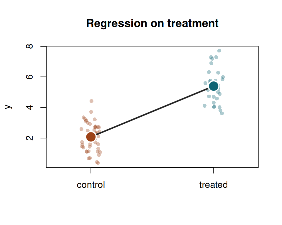
**Simulation — treatment alone.** Regress $y$ on the treatment $D$ alone — here 30 treated drawn $y \sim N(5, 1)$ and 50 controls $y \sim N(2, 1)$. The residual $\tilde V_i = D_i - \bar D$ is constant within each group, so the weight is uniform within a group and $\hat\beta$ reduces to the two group means: $\hat\beta = \bar y_1 - \bar y_0$, the difference in means. Every treated unit then carries positive weight, every control negative — the structural pattern of the previous section, with the wrong-sign off-diagonal empty until covariates enter.
```{r}
#| fig-width: 5
#| fig-height: 4
#| fig-cap: "Regression on the treatment alone. Points are the two groups (rust control, teal treated); the large dots are the group means, and the segment joining them has slope $\\hat\\beta = \\bar y_1 - \\bar y_0$, the difference in means."
set.seed(7)
n1 <- 30; n0 <- 50
d <- c(rep(1, n1), rep(0, n0)); y <- c(rnorm(n1, 5), rnorm(n0, 2))
dev <- d - mean(d); om <- dev / sum(dev^2); col <- ifelse(om >= 0, teal, rust)
y1 <- mean(y[d == 1]); y0 <- mean(y[d == 0])
plot(jitter(d, 0.4), y, pch = 16, col = paste0(col, "55"), cex = 0.9,
     xlim = c(-0.3, 1.3), xaxt = "n", xlab = "", ylab = "y", main = "Regression on treatment")
axis(1, at = c(0, 1), labels = c("control", "treated"))
segments(0, y0, 1, y1, lwd = 2.6, col = "grey15")
points(c(0, 1), c(y0, y1), pch = 21, bg = c(rust, teal), col = "white", cex = 2.5, lwd = 2)
vtab(c(`$\\hat\\beta$ (lm)` = coef(lm(y ~ d))[["d"]], `$\\bar y_1 - \\bar y_0$` = y1 - y0,
        `off-diagonal weights` = sum((d == 1 & om < 0) | (d == 0 & om > 0))), 3)
```
The estimate equals $\bar y_1 - \bar y_0$, and no weight carries the wrong sign — the off-diagonal count is zero.
**Simulation — 2×2 difference-in-differences.** Add a period and interact it with the group, and the design has four cells. Each collapses to its mean, and the interaction coefficient is their double contrast,
$$ \widehat{\text{DiD}} = (\bar y_{T,\text{post}} - \bar y_{T,\text{pre}}) - (\bar y_{C,\text{post}} - \bar y_{C,\text{pre}}). $$ {#eq-outcome-weights-11}
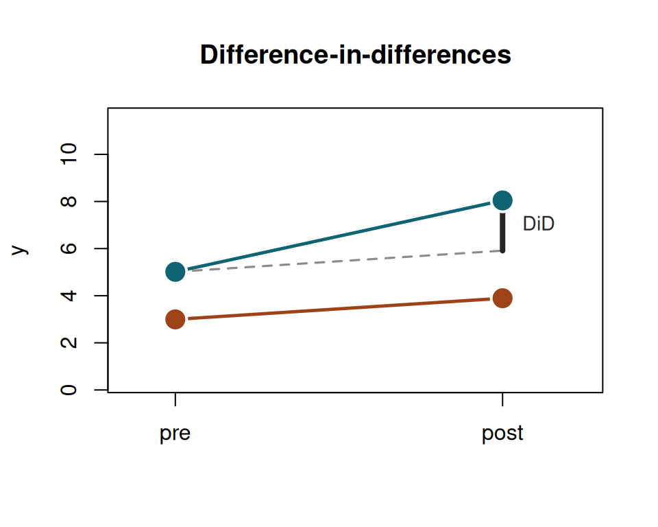
Now there are four cell means, and with them four slopes — the two group trends over time and the two cross-sectional gaps. The DiD is the difference between either parallel pair, trend minus trend or gap minus gap. We simulate 200 units in each group×period cell from $y = 3 + 2g + p + 2\,(g \cdot p) + \varepsilon$ with $\varepsilon \sim N(0,1)$, so the true DiD (the interaction) is $2$:
```{r}
#| fig-width: 5
#| fig-height: 4
#| fig-cap: "The 2×2 difference-in-differences: four cell means (dots), the treated (teal) and control (rust) trends, the parallel-trends counterfactual (dashed), and the DiD (black bar) as the gap between the treated post-mean and that counterfactual."
set.seed(3)
g <- rep(c(1, 1, 0, 0), each = 200); p <- rep(c(0, 1, 0, 1), each = 200)
y <- 3 + 2 * g + 1 * p + 2 * (g * p) + rnorm(800)
m <- tapply(y, list(g, p), mean)
Tpre <- m["1", "0"]; Tpost <- m["1", "1"]; Cpre <- m["0", "0"]; Cpost <- m["0", "1"]
cf <- Tpre + (Cpost - Cpre)
plot(NA, xlim = c(-0.15, 1.25), ylim = range(y), xaxt = "n", xlab = "", ylab = "y",
     main = "Difference-in-differences")
axis(1, at = c(0, 1), labels = c("pre", "post"))
segments(0, Tpre, 1, Tpost, lwd = 2.4, col = teal)
segments(0, Cpre, 1, Cpost, lwd = 2.4, col = rust)
segments(0, Tpre, 1, cf, lty = 2, lwd = 1.6, col = "grey55")
segments(1, cf, 1, Tpost, lwd = 4, col = "grey15")
points(c(0, 1, 0, 1), c(Tpre, Tpost, Cpre, Cpost),
       pch = 21, bg = c(teal, teal, rust, rust), col = "white", cex = 2.3, lwd = 2)
text(1.02, (cf + Tpost) / 2, "DiD", pos = 4, cex = 0.9, col = "grey15")
vtab(c(`treated trend` = Tpost - Tpre, `control trend` = Cpost - Cpre,
        `pre gap` = Tpre - Cpre, `post gap` = Tpost - Cpost,
        `DiD (interaction)` = coef(lm(y ~ g * p))[["g:p"]]), 3)
```
The estimated interaction recovers the true DiD of $2$, and the four cell-mean weights carry the structural signs $(+, -, -, +)$ as long as every cell is populated.
The clean $2 \times 2$ has trivial weights — four cell means, each $\pm 1$. Real difference-in-differences carries covariates: parallel trends holds only *conditional* on $X$, and the comparison has to be modelled. That model is a weighting of outcomes too.
The doubly-robust DiD of Sant'Anna and Zhao (2020) is AIPW read on the outcome *change* $\Delta Y = Y_1 - Y_0$: a propensity for treatment, a control-group regression of $\Delta Y$ on $X$, combined. By the recipe of the last section its estimate is $\widehat{\text{ATT}} = \boldsymbol\omega' \Delta Y$, with $\boldsymbol\omega' = \boldsymbol a'(\mathbf I - \boldsymbol S)$ — the control-trend smoother $\boldsymbol S$ and the group weights $\boldsymbol a = \boldsymbol w_{\text{treat}} - \boldsymbol w_{\text{cont}}$.
**Simulation — doubly-robust DiD.** Two periods and $n = 2000$, with covariates $x_1, x_2 \sim N(0,1)$. Treatment is selected on $x_1$ with thin overlap, $\Pr(D = 1) = \Lambda(-0.5 + 2 x_1)$. The outcomes are $y_{i0} = 1 + x_{1i} + 0.5\,x_{2i} + \varepsilon_{i0}$ and $y_{i1} = y_{i0} + (0.5 + 0.4\,x_{1i}) + D_i + \varepsilon_{i1}$, with both errors $N(0,1)$. The control trend $0.5 + 0.4 x_1$ depends on $x_1$, so trends are parallel only given $X$, and the true ATT is $1$. We fit DR-DiD with `DRDID`, rebuild its weights by hand, and check.
```{r}
#| message: false
#| warning: false
library(DRDID)
set.seed(2)
n  <- 2000
x1 <- rnorm(n); x2 <- rnorm(n); Xcov <- cbind(1, x1, x2)
D  <- rbinom(n, 1, plogis(-0.5 + 2 * x1))        # selection into treatment on x1 (thin overlap)
y0 <- 1 + x1 + 0.5 * x2 + rnorm(n)               # pre-period outcome
y1 <- y0 + (0.5 + 0.4 * x1) + 1 * D + rnorm(n)   # control trend depends on x1; true ATT = 1
dY <- y1 - y0
att <- drdid_panel(y1 = y1, y0 = y0, D = D, covariates = Xcov, boot = FALSE)$ATT

# rebuild the DR-DiD weights: omega = (I - S)' a, acting on the outcome change dY
e    <- pmin(as.vector(glm(D ~ x1 + x2, family = binomial)$fitted), 1 - 1e-6)
keep <- rep(TRUE, n); keep[D == 0] <- e[D == 0] < 0.995     # DRDID's control trimming
Xc   <- Xcov[D == 0, ]
S    <- matrix(0, n, n); S[, D == 0] <- Xcov %*% solve(crossprod(Xc)) %*% t(Xc)
w.t  <- keep * D
w.c  <- keep * e * (1 - D) / (1 - e)
a    <- w.t / sum(w.t) - w.c / sum(w.c)          # group weights, treated minus reweighted control
omega <- as.vector(a - crossprod(S, a))

Xk <- cbind(x1, x2); sds <- apply(Xk, 2, sd)
vtab(c(`DRDID ATT`                = att,
       `$\\boldsymbol\\omega'\\Delta\\boldsymbol Y$`                = sum(omega * dY),
       `wrong-sign weights`       = sum((D == 1 & omega < 0) | (D == 0 & omega > 0)),
       `covariate imbalance, raw` = max(abs((colMeans(Xk[D == 1, ]) - colMeans(Xk[D == 0, ])) / sds)),
       `covariate imbalance, wtd` = max(abs(as.vector(a %*% Xk) / sds))), 3)
```
$\boldsymbol\omega' \Delta Y$ reproduces the `DRDID` estimate exactly — the difference-in-differences is a signed weighting of observed outcome *changes*, and the diagnostics of this chapter apply to it. The weighting balances the covariate that drove selection (its standardised imbalance falls from $1.20$ to $0.09$). And $151$ units carry a wrong-sign weight — a treated unit subtracted, or a control added — the signature of a comparison reaching past common support.
### Staggered designs: TWFE at the observation level
Negative weights in staggered designs are usually described at the level of two-by-two comparisons: TWFE averages many such comparisons, and some enter with a negative weight — the forbidden comparisons that use already-treated units as controls (de Chaisemartin and D'Haultfœuille 2020; Goodman-Bacon 2021). That is the effect-weight reading. The outcome-weight reading goes one level down, to the individual $y_{it}$.
TWFE is still FWL: residualise $D_{it}$ on unit and time fixed effects to get $\tilde D_{it}$, and $\hat\beta = \sum_{it} \omega_{it} y_{it}$ with $\omega_{it} = \tilde D_{it} / \sum_{jt} \tilde D_{jt}^2$. A treated observation with $\omega_{it} < 0$ is a cell whose outcome is subtracted from the estimated effect — used as a control even though it is treated. An untreated observation with $\omega_{it} > 0$ enters as though it were treated. Both are the same sign flip seen earlier under thin overlap, caused here by the unit-and-time residualisation pushing $\tilde D_{it}$ past zero: treated cells in late periods of early cohorts, where the fixed-effect prediction of $D_{it}$ exceeds $1$, and untreated cells in early periods of never-treated units, where it falls below $0$.
**Simulation — staggered panel.** $N = 300$ units over $T = 8$ periods, in three cohorts: never-treated ($20\%$), early-treated at period $3$ with effect $\tau = 3$ ($40\%$), and late-treated at period $6$ with effect $\tau = 1$ ($40\%$). Outcomes are $y_{it} = \alpha_i + \gamma_t + \tau_g D_{it} + \varepsilon_{it}$, with unit effects $\alpha_i \sim N(0,1)$, a time effect $\gamma_t$ rising linearly from $0$ to $1.4$, and $\varepsilon_{it} \sim N(0, 0.5^2)$. The high treated share makes the forbidden comparison visible.
```{r}
#| message: false
library(fixest)
set.seed(5)
N <- 300; TT <- 8
g <- sample(c(0, 3, 6), N, TRUE, prob = c(.2, .4, .4))
panel <- data.frame(id = rep(1:N, each = TT), t = rep(1:TT, N))
panel$g <- g[panel$id]
panel$D <- as.integer(panel$g > 0 & panel$t >= panel$g)
tau <- ifelse(panel$g == 3, 3, ifelse(panel$g == 6, 1, 0))
alpha <- rnorm(N); gamma <- seq(0, 1.4, length.out = TT)
panel$y <- alpha[panel$id] + gamma[panel$t] + tau * panel$D + rnorm(nrow(panel), 0, 0.5)

Dtil <- resid(feols(D ~ 1 | id + t, data = panel))
omega_tw <- Dtil / sum(Dtil^2)
n1 <- sum(panel$D)
vtab(c(`true ATT`              = mean(tau[panel$D == 1]),
       `TWFE`                  = coef(feols(y ~ D | id + t, panel))[["D"]],
       `$\\boldsymbol\\omega'\\boldsymbol y$`              = sum(omega_tw * panel$y),
       `treated, $\\omega_i < 0$`    = sum(panel$D == 1 & omega_tw < 0),
       `untreated, $\\omega_i > 0$`  = sum(panel$D == 0 & omega_tw > 0)), 3)
```
The TWFE coefficient sits well below the true ATT, and $\sum \omega_{it} y_{it}$ reproduces it exactly. Hundreds of treated cells carry a negative weight: these are the early cohort's cells in periods $6$–$8$, the ones where the unit-and-time prediction of $D$ exceeds $1$ and the residual $\tilde D_{it}$ flips sign. Their outcomes are subtracted from $\hat\beta$ — the observation-level signature of the Bacon forbidden comparison.
The wrong-sign diagnostic in a panel is by observation $(i, t)$, not by unit. In the cross-sectional case earlier, the fix was to trim wrong-sign observations and refit. In a panel, trimming specific $(i, t)$ cells removes observations that anchor that unit's fixed effect and distorts the estimates for its remaining cells. The response in the staggered setting is to switch estimators — imputation (Borusyak, Jaravel, and Spiess 2024), Callaway and Sant'Anna, or Sun and Abraham — that avoid the forbidden comparison by construction. The imputation estimator, for example, fits unit and time fixed effects on untreated observations alone and imputes each treated cell's counterfactual; because its smoother draws only on untreated outcomes, the weight on every treated cell reduces to $1/n_1$ and no treated observation can count as a control.
### Synthetic difference-in-differences: a rank-one weighting
Synthetic difference-in-differences is a weighted two-way fixed effects regression, from Arkhangelsky, Athey, Hirshberg, Imbens, and Wager (2021). The estimators so far imply their weights. This one chooses them:
$$ (\hat\tau, \hat\mu, \hat\alpha, \hat\beta) = \arg\min \sum_{i}\sum_{t} \big(Y_{it} - \mu - \alpha_i - \beta_t - W_{it}\tau\big)^2\, \omega_i \lambda_t. $$ {#eq-outcome-weights-12}
The recipe: fit $\omega_i$ on the control units so the reweighted control path tracks the treated path over the pre-period, and fit $\lambda_t$ on the pre-periods so the reweighted pre-period resembles the post-period. Treated units enter at $1/N_1$, post-periods at $1/T_1$. Both fitted sets lie on the simplex, non-negative and summing to one.
@eq-outcome-weights-12 is weighted least squares, so the FWL reading of @eq-omega goes through with the weights carried along. Then $\hat\tau$ is again a weighting of outcomes. Let $u_i$ be $1/N_1$ for a treated unit and $-\omega_i$ for a control. Let $v_t$ be $1/T_1$ for a post-period and $-\lambda_t$ for a pre-period. Then
$$ \hat\tau = \sum_i \sum_t \omega_{it}\, Y_{it}, \qquad \omega_{it} = u_i \, v_t. $$ {#eq-outcome-weights-13}
In words, the weight on a cell is a unit part times a time part. Collect the weights into an $N \times T$ matrix $\boldsymbol\Omega$, one entry per cell. Then @eq-outcome-weights-13 reads $\boldsymbol\Omega = \boldsymbol u \boldsymbol v'$, an outer product, and a matrix of that form has **rank one**. Every row is a multiple of every other row. So each unit carries the same weight profile over time, scaled by its own $u_i$, and each period weights the units in the same pattern, scaled by its own $v_t$. There is no unit-by-period interaction in the weights.
That product structure is what makes this a difference-in-differences. A double difference contrasts units and contrasts periods, and multiplying the two contrasts gives a rank-one weighting. We come back to the rank below, where it separates the block designs from the staggered ones.
Multiply @eq-outcome-weights-13 out and we get the $2 \times 2$ of @eq-outcome-weights-11 with two of its four averages reweighted, the control average by $\omega$ and the pre-period average by $\lambda$:
$$ \hat\tau = \Big(\bar Y_{T,\text{post}} - \sum_{t \in \text{pre}} \lambda_t \bar Y_{T,t}\Big) - \Big(\sum_{i \in C} \omega_i \bar Y_{i,\text{post}} - \sum_{i \in C}\sum_{t \in \text{pre}} \omega_i \lambda_t Y_{it}\Big). $$ {#eq-outcome-weights-14}
The four blocks keep the signs $(+, -, -, +)$ of @eq-outcome-weights-11. Only the averages inside two of them change, and they are no longer uniform.
**Simulation — the outcome weights of synthetic DiD.** A panel of $40$ control and $10$ treated units over $12$ pre- and $6$ post-periods. Untreated outcomes are
$$ Y_{it}(0) = \alpha_i + \beta_t + \boldsymbol f_i' \boldsymbol g_t + \varepsilon_{it}, $$ {#eq-factor-dgp}
with a unit effect $\alpha_i \sim N(0, 0.5^2)$, a time effect $\beta_t$ rising linearly from $0$ to $1$, two factors in $\boldsymbol g_t$ (one linear in $t$, one a sine), loadings $\boldsymbol f_i \sim N(\boldsymbol 0, \mathbf I)$ shifted by $0.8$ for the treated units, and $\varepsilon_{it} \sim N(0, 0.3^2)$. The spread in $\boldsymbol f_i$ makes the control trends differ from each other, and the shift makes the treated trend differ from all of them. The true ATT is $2$. We fit with `synthdid`, then rebuild @eq-outcome-weights-13 by hand from the fitted $\omega$ and $\lambda$.
```{r}
library(synthdid)
set.seed(11)
N0 <- 40; N1 <- 10; N <- N0 + N1; T0 <- 12; T1 <- 6; Tt <- T0 + T1
f <- cbind(rnorm(N), rnorm(N)); f[(N0 + 1):N, ] <- f[(N0 + 1):N, ] + 0.8
g <- cbind(seq(0, 2, length = Tt), sin(seq(0, 3, length = Tt)))
Y <- outer(rnorm(N, 0, .5), rep(1, Tt)) + outer(rep(1, N), seq(0, 1, length = Tt)) +
     f %*% t(g) + matrix(rnorm(N * Tt, 0, .3), N, Tt)
W <- matrix(0, N, Tt); W[(N0 + 1):N, (T0 + 1):Tt] <- 1
Y <- Y + 2 * W                                          # true ATT = 2

est <- synthdid_estimate(Y, N0, T0)
wt  <- attr(est, "weights")
u <- c(-wt$omega,  rep(1 / N1, N1))                     # unit part
v <- c(-wt$lambda, rep(1 / T1, T1))                     # time part
Omega <- outer(u, v)                                    # outcome weight on cell (i, t)
```
Three routes should give the same number: what `synthdid` reports, the weighting @eq-outcome-weights-13 applies to the observed outcomes, and the weighted regression of @eq-outcome-weights-12.
```{r}
cw <- outer(c(wt$omega, rep(1 / N1, N1)), c(wt$lambda, rep(1 / T1, T1)))
dd <- data.frame(y = as.vector(Y), Wt = as.vector(W), i = factor(rep(1:N, Tt)),
                 t = factor(rep(1:Tt, each = N)), cw = as.vector(cw))
tau3 <- c(`synthdid_estimate()`              = as.numeric(est),
          `$\\sum_{it} \\omega_{it} Y_{it}$, by hand` = sum(Omega * Y),
          `weighted TWFE regression`        = coef(lm(y ~ Wt + i + t, dd,
                                                      weights = dd$cw))[["Wt"]])
vtab(c(tau3, `largest gap between them` = max(abs(tau3 - tau3[1]))), 6)
```
The gap between them is zero to machine precision. The outer-product form is what `synthdid` computes.
Writing the weights this way puts three constraints on them. First, the rank is one, since a cell's weight is a unit part times a time part. Second, each margin sums to zero on its own: $\omega$ and $\lambda$ each sum to one, and the treated and post-period blocks each contribute an offsetting one. Third, no cell carries a wrong sign: no treated post-period cell is subtracted, and no control pre-period cell is added. We check all three.
```{r}
chk <- rbind(`rank of $\\boldsymbol\\Omega$`     = c(sum(svd(Omega)$d > 1e-12), 1),
             `$\\sum_i u_i$`     = c(sum(u), 0),
             `$\\sum_t v_t$`   = c(sum(v), 0),
             `treated post-cells, $\\omega_{it} < 0$` = c(sum(Omega[(N0+1):N, (T0+1):Tt] < 0), 0),
             `control pre-cells, $\\omega_{it} < 0$`  = c(sum(Omega[1:N0, 1:T0] < 0), 0))
colnames(chk) <- c("found", "should be")
mtab(chk, 4)
```
All three hold. Note that the double zero-sum is stronger than the single sum-to-zero of @eq-omega, which constrains the weights only in total. Here they vanish along each margin. The signs are fixed by construction too: a treated post-period cell gets $1/(N_1 T_1) > 0$, and a control pre-period cell gets $\omega_i \lambda_t > 0$, because the simplex rules out a negative $\omega_i$. The doubly-robust fit above produced $151$ wrong-sign units. Synthetic DiD cannot produce any.
The remaining question is how much of the panel the comparison uses. Counting the non-zero weights is one answer, but it treats a weight of $0.4$ and a weight of $0.001$ alike. The usual summary that does not is the **effective sample size**, and it is worth deriving rather than asserting. Take $m$ observations with equal variance $\sigma^2$. An unweighted mean of them has variance $\sigma^2/m$. A weighted mean with weights $w$ summing to one has variance $\sigma^2 \sum w^2$. Ask which $m$ makes the two equal:
$$ \frac{\sigma^2}{m} = \sigma^2 \sum_j w_j^2 \qquad\Longrightarrow\qquad m = \frac{1}{\sum_j w_j^2}. $$ {#eq-ess}
So @eq-ess is the number of equally weighted observations that would deliver the same precision as the weighting actually used. It equals the full count when every weight is equal, and $1$ when one observation carries everything. We apply it to each margin separately: to the control weights as $1/\sum_i \omega_i^2$, and to the pre-period weights as $1/\sum_t \lambda_t^2$. Both are sparse here, so both fall below the nominal $40$ controls and $12$ pre-periods.
```{r}
dsg <- c(sum(wt$omega > 1e-8), 1 / sum(wt$omega^2),
         sum(wt$lambda > 1e-8), 1 / sum(wt$lambda^2), wt$lambda[T0])
names(dsg) <- c(sprintf("controls with non-zero weight (of %d)", N0),
                sprintf("effective controls, $1/\\sum_i \\omega_i^2$ (of %d)", N0),
                sprintf("pre-periods with non-zero weight (of %d)", T0),
                sprintf("effective pre-periods, $1/\\sum_t \\lambda_t^2$ (of %d)", T0),
                "weight on the last pre-period")
vtab(dsg)
```
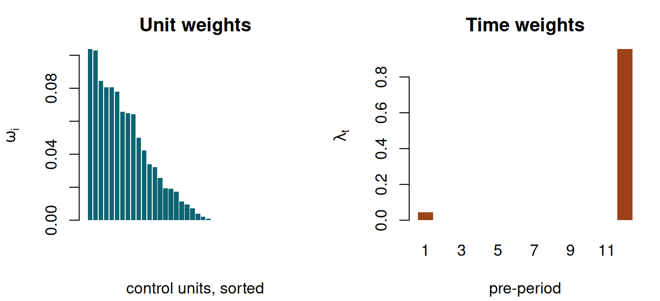
Only $23$ of the $40$ controls get any weight, and the effective count is $14.6$. Three reference points make that number readable. Weighting all $40$ equally would give $40$, and that is plain difference-in-differences. Weighting the $23$ active controls equally, at $1/23$ each, would give $23$. The comparison actually delivers $14.6$, so the drop from $23$ to $14.6$ measures nothing but the inequality among those $23$ weights: a few carry most of the mass and the rest contribute little.
A larger effective size is not automatically better, and it is worth seeing why. By Cauchy–Schwarz, $\sum_i \omega_i^2 \ge 1/N_0$ with equality only when every weight equals $1/N_0$, so the effective size reaches $N_0$ exactly when the weighting is uniform — that is, when no reweighting has happened. Matching the treated path requires tilting toward the controls that resemble it, and any tilt lowers the effective size. The two things we want pull against each other, and the effective count is the price paid for the match rather than a score to be maximised. The one case where both arrive together is when the treated path already equals the unweighted control average, and then there was nothing to reweight for.
Synthetic difference-in-differences prices that trade-off explicitly, which is why the effective count is the number to read. Its weights minimise not the pre-period fit alone but
$$ (\text{pre-period fit error}) \; + \; \zeta^2 \sum_i \omega_i^2 , $$ {#eq-sdid-penalty}
and by @eq-ess the penalty $\zeta^2 \sum_i \omega_i^2$ is exactly $\zeta^2$ divided by the effective sample size. So the estimator charges itself for concentration at a rate $\zeta$, which by default rises with the estimated noise in the panel: noisier data is shrunk harder toward uniform, because in noisy data an apparent gain from concentrating is more likely to be fitted noise. The $14.6$ above is where that trade-off settled on this panel, and it is computable whether or not we know what generated the data. The time margin is sparser: an effective $1.09$ pre-periods, with $0.957$ of the mass on the last one. The counterfactual level is anchored on the single period before treatment, so the estimate inherits that period's noise. We can read all of this off the weights. None of it is visible in $\hat\tau$.
We plot the two margins to see where the mass sits. The left panel sorts the fitted control weights $\omega_i$ from largest to smallest, which shows how many controls the comparison uses. The right panel keeps the pre-period weights $\lambda_t$ in time order, which shows which periods the counterfactual is built from.
```{r}
#| fig-width: 7
#| fig-height: 3.2
#| fig-cap: "The two margins of the synthetic DiD weight matrix. Left: fitted control-unit weights $\\omega_i$, sorted. $23$ of $40$ are non-zero, and the $17$ the simplex sets to zero lie flat against the axis. Right: fitted pre-period weights $\\lambda_t$. Almost all the mass is on the last pre-period, so the counterfactual level is anchored just before treatment."
par(mfrow = c(1, 2), mar = c(4.2, 4.2, 2.6, 1))
os <- sort(wt$omega, decreasing = TRUE)
barplot(os, col = ifelse(os > 1e-8, teal, "grey85"), border = NA,
        xlab = "control units, sorted", ylab = expression(omega[i]),
        main = "Unit weights")
barplot(wt$lambda, names.arg = 1:T0, border = NA,
        col = ifelse(wt$lambda > 1e-8, rust, "grey85"),
        xlab = "pre-period", ylab = expression(lambda[t]), main = "Time weights")
```
### The rank of the weight matrix
Synthetic difference-in-differences has a rank-one $\boldsymbol\Omega$ by construction. So does the plain $2 \times 2$: set $u_i$ and $v_t$ to the uniform $\pm 1/N_g$ and $\pm 1/T_g$ and @eq-outcome-weights-11 reappears. Staggered adoption gives a higher rank, bounded by the number of cohorts.
Write the staggered treatment matrix as a sum over adoption cohorts, $\boldsymbol W = \sum_{k=1}^{K} \boldsymbol c_k \boldsymbol s_k'$. Here $\boldsymbol c_k$ indicates the units of cohort $k$, and $\boldsymbol s_k$ the periods from its adoption date on. That is a sum of $K$ rank-one terms. Residualising on unit and time dummies is a double centring, $(\mathbf I - \boldsymbol P)\, \boldsymbol W \,(\mathbf I - \boldsymbol Q)$, and double centring cannot raise a rank. So $\operatorname{rank}(\boldsymbol\Omega) \le K$, with equality generically.
We check the bound directly. Each panel has $60$ units over $20$ periods, with one to five adoption dates plus a never-treated group. For each we build the staggered TWFE weights, then count the non-zero singular values of $\boldsymbol\Omega$.
```{r}
set.seed(4)
Ns <- 60; Ts <- 20
rk <- sapply(list(10, c(8, 14), c(6, 10, 14), c(6, 9, 12, 15), c(5, 8, 11, 14, 17)),
  function(dates) {
    coh <- sample(c(dates, Inf), Ns, replace = TRUE)     # Inf = never treated
    Ws  <- matrix(0, Ns, Ts)
    for (i in 1:Ns) if (is.finite(coh[i])) Ws[i, coh[i]:Ts] <- 1
    ds  <- data.frame(Wt = as.vector(Ws), i = factor(rep(1:Ns, Ts)),
                      t = factor(rep(1:Ts, each = Ns)))
    Wtil <- residuals(lm(Wt ~ i + t, ds))
    Om   <- matrix(Wtil / sum(Wtil^2), Ns, Ts)
    c(`treated cohorts` = length(dates),
      `rank of $\\boldsymbol\\Omega$`   = sum(svd(Om)$d > 1e-9 * max(svd(Om)$d)))
  })
colnames(rk) <- c("1 date", "2 dates", "3 dates", "4 dates", "5 dates")
mtab(rk)
```
The rank is at most the number of treated cohorts, and equals it generically. This ties the chapter's difference-in-differences material together. A block design has one adoption date, so its weight matrix is rank one. The plain $2 \times 2$ and synthetic difference-in-differences are the same object at two settings of the margins, uniform in the first and fitted in the second. Staggered adoption raises the rank. Once a cell's weight no longer factors into a unit part times a time part, a treated cell can enter negatively. In the block case it cannot, since every treated post-period cell gets $u_i v_t = 1/(N_1 T_1) > 0$. The forbidden comparisons need the extra rank.
### Which margin does the work
The weight matrix has two margins, $\boldsymbol u$ over units and $\boldsymbol v$ over periods, and @eq-outcome-weights-13 says the whole weighting is their product. So a natural question about the structure is which margin carries the correction when the control trends differ from the treated group's.
It is worth saying first what such a correction can and cannot be. Parallel trends is a statement about two group means, $E[\Delta Y(0) \mid D = 1] = E[\Delta Y(0) \mid D = 0]$, and no single observation either has it or lacks it, so in the model behind @eq-outcome-weights-11 there is nothing at the unit level for a weight to act on. Weighting bites only under a model where trends vary across units: unit-specific slopes, or a factor structure. Then each unit has its own trend, and reweighting controls toward those whose loadings resemble the treated group's is well defined. That is what synthetic difference-in-differences does, and what the wider family of trajectory-balancing and history-matching estimators does too (Hazlett and Xu 2018; Imai, Kim, and Wang 2023; Doudchenko and Imbens 2016).
We can then hold one margin uniform and fit the other, and read off how much of the correction each supplies.
**Simulation — which margin does the work.** Two panels of $40$ controls and $10$ treated over $12$ pre- and $6$ post-periods, with a true ATT of $2$. Both carry a unit effect $\alpha_i \sim N(0,1)$, shifted up by $1$ for the treated units, a time effect $\beta_t$ rising linearly from $0$ to $1.5$, and a serially correlated shock. The shock is a stationary AR(1),
$$ \varepsilon_{it} = \rho\, \varepsilon_{i,t-1} + \nu_{it}, \qquad \nu_{it} \sim N(0, \sigma^2), \qquad \rho = 0.5, $$ {#eq-ar1}
started from its stationary distribution, so $\varepsilon_{it}$ has standard deviation $\sigma/\sqrt{1 - \rho^2}$. We set $\sigma = 0.4$, which makes the shock's own standard deviation $0.46$. Note the distinction: $\sigma$ is the standard deviation of the innovation $\nu_{it}$ that arrives each period, not of the shock $\varepsilon_{it}$ that accumulates.
The shock is serially correlated rather than independent for a reason, and it is not decoration. The weights are fitted on the pre-period path. Under independent noise, averaging across twelve pre-periods removes most of it, so the weights would recover the systematic path almost exactly and there would be little left to study. Serial correlation means twelve periods carry well under twelve periods' worth of independent information, and that is what leaves the fitted weights short. It is also the realistic case: panel outcomes persist. AR(1) is the smallest model with a persistence parameter, nesting independent noise at $\rho = 0$ and a random walk as $\rho \to 1$.
These three terms are common to almost any panel, and none of them breaks parallel trends: $\alpha_i$ differences away and $\beta_t$ is shared by both groups, so a difference-in-differences removes them whatever the weights are.
Parallel trends fails only when the treated and control groups have *different* untreated trends, so a term that varies by unit and moves with $t$ is what we have to put in. Without one there is nothing for the weights to fix. The two panels are two forms of it. The `factor` panel uses the $\boldsymbol f_i' \boldsymbol g_t$ of @eq-factor-dgp. The `slopes` panel replaces it with a unit-specific linear trend,
$$ Y_{it}(0) = \alpha_i + \beta_t + s_i \, t + \varepsilon_{it}, \qquad s_i \sim N(0,\, 0.08^2), $$ {#eq-slopes-dgp}
with $s_i$ shifted up by $0.12$ for the treated units. So each unit has its own growth rate, and the treated units grow faster on average, by about one and a half standard deviations of the control slopes. Note that $s_i t$ is itself a one-factor model, with loading $s_i$ and factor $g_t = t$. It is the simplest member of the class @eq-factor-dgp describes, which is the class synthetic difference-in-differences is built for, so this is a leading case and not a special one. We run synthetic DiD four ways: both margins uniform, which is plain difference-in-differences; unit weights fitted with time weights uniform; time weights fitted with unit weights uniform; and both fitted. $400$ replications.
```{r}
library(parallel)
panel <- function(kind, N0 = 40, N1 = 10, T0 = 12, T1 = 6, sig = .4, rho = .5) {
  N <- N0 + N1; Tt <- T0 + T1
  a <- rnorm(N, 0, 1); a[(N0 + 1):N] <- a[(N0 + 1):N] + 1
  e <- matrix(0, N, Tt); e[, 1] <- rnorm(N, 0, sig / sqrt(1 - rho^2))
  for (t in 2:Tt) e[, t] <- rho * e[, t - 1] + rnorm(N, 0, sig)
  Y0 <- outer(a, rep(1, Tt)) + outer(rep(1, N), seq(0, 1.5, length = Tt)) + e
  if (kind == "factor") {
    f <- cbind(rnorm(N), rnorm(N)); f[(N0 + 1):N, ] <- f[(N0 + 1):N, ] + 0.8
    g <- cbind(seq(0, 2, length = Tt), sin(seq(0, 3, length = Tt)))
    Y0 <- Y0 + f %*% t(g)
  } else {
    s <- rnorm(N, 0, .08); s[(N0 + 1):N] <- s[(N0 + 1):N] + .12   # unit slopes
    Y0 <- Y0 + outer(s, 1:Tt)
  }
  W <- matrix(0, N, Tt); W[(N0 + 1):N, (T0 + 1):Tt] <- 1
  list(Y = Y0 + 2 * W, N0 = N0, N1 = N1, T0 = T0, T1 = T1)
}
margins <- function(r, kind) {
  set.seed(5000 + r); p <- panel(kind); N0 <- p$N0; T0 <- p$T0
  fx <- function(om, lam) as.numeric(synthdid_estimate(p$Y, N0, T0,
          weights = list(omega = om, lambda = lam)))     # NULL = fit this margin
  unif.o <- rep(1 / N0, N0); unif.l <- rep(1 / T0, T0)
  c(`both uniform (DiD)` = fx(unif.o, unif.l), `unit weights only` = fx(NULL, unif.l),
    `time weights only`  = fx(unif.o, NULL),   `both fitted (SDID)` = fx(NULL, NULL))
}
res <- lapply(c("factor", "slopes"), function(kind) {
  # portable core count: mclapply falls back to serial on Windows
  n_cores <- if (.Platform$OS.type == "windows") 1L else
               max(1L, min(6L, parallel::detectCores() - 1L))
  M <- simplify2array(mclapply(1:400, margins, kind = kind, mc.cores = n_cores))
  cbind(bias = rowMeans(M) - 2, sd = apply(M, 1, sd), rmse = sqrt(rowMeans((M - 2)^2)))
})
out <- cbind(res[[1]], res[[2]])
colnames(out) <- paste(rep(c("factor", "slopes"), each = 3), colnames(res[[1]]))
mtab(out)
```
Reweighting helps, and by a lot. Under the factor structure the bias falls from $0.73$ to $0.04$ with both margins fitted. Each margin helps alone: $0.17$ from the unit weights, $0.08$ from the time weights. Which margin matters is not fixed in advance. Here the time weights do slightly more, because the factor paths are smooth, so anchoring on the periods just before treatment removes most of the divergence. The fitted $\lambda$ above showed the same thing when it put $0.957$ on the last pre-period.
The `slopes` panel gains less: $1.08$ down to $0.40$. The reason is that the weights are fitted on the observed pre-period path, which carries the shock of @eq-ar1 as well as the trend, so they match a noisy version of what they are aiming at and fall short. The size of that shortfall depends on the pre-period length and the noise level rather than on anything intrinsic to reweighting — with a much cleaner pre-period the same estimator gets the bias under $0.05$ — so the direction is the finding here and the magnitude is not.
Two limits are worth stating even though they do not bind in this panel. Reweighting controls can only produce a weighted average of the control trends, so a treated trend steeper than every control's is out of reach; that is the same overlap problem seen earlier, now in the design, and the simplex is what makes it a hard boundary rather than a silent extrapolation. And if we are confident the trends really are unit-specific and linear, the direct response is to put unit-specific linear trends in the regression, not to reweight at all. Reweighting is the tool for when we will not commit to a functional form, which is the case @eq-factor-dgp stands in for.
### Implied versus chosen
One distinction cuts across everything above. OLS, AIPW, DML, TWFE, and the imputation estimator all *imply* weights — they fall out of the estimation and are diagnosed afterward. Synthetic controls and synthetic difference-in-differences *choose* weights as part of the design, selecting $\boldsymbol\omega$ to balance pre-treatment outcomes or covariates. For those estimators $\hat\tau = \boldsymbol\omega'\boldsymbol Y$ is the definition, not a decomposition.
That difference changes how the weights should be read, in three ways. First, chosen weights are fitted on $\boldsymbol Y$ itself, so $\hat\tau$ is not linear in $\boldsymbol Y$ and @eq-outcome-weights-13 describes the estimate at the fitted weights rather than decomposing it the way @eq-omega decomposes OLS. Inference has to account for the weights having been estimated, which is why `synthdid` reports standard errors by jackknife or bootstrap rather than treating $\boldsymbol\omega$ as fixed.
Second, a clean-looking balance diagnostic is weaker evidence here than it looks. When the weights were chosen to make the pre-period match, the match is not a test the design passed — it is what the design optimised. Fitting weights on a noisy pre-period statistic is a close cousin of a pretest. The analogy is with Roth (2022), who shows that conditioning an analysis on passing a parallel-trends test distorts the estimate and undercovers. Weight-fitting is not literally that procedure, since nothing is accepted or rejected, but it shares the mechanism: noise in the pre-period is allowed to select the analysis. Matching on pre-period *levels* is the sharp case: it induces regression to the mean, with a bias that grows as serial correlation weakens (Daw and Hatfield 2018; Chabé-Ferret 2015, 2017). Synthetic difference-in-differences avoids that particular trap by fitting $\boldsymbol\omega$ with an intercept, so it never needs to match levels, only trajectories up to a constant.
Third, the effective count of @eq-ess is the number that reports the price. A design that matches well by concentrating weight on a few controls has bought that match with effective sample size, and @eq-sdid-penalty shows the estimator charging itself for exactly that. Read the two together rather than either alone.
A closing caution. These weights diagnose estimation. They show which comparisons a difference-in-differences rests on, and whether it uses non-overlapping or forbidden ones. They do not test identification. Parallel trends is an assumption about the treated group's unobserved untreated path, and a negative weight and a failure of parallel trends stay independent: either can occur without the other. Chosen weights can buy robustness to one class of violations, those the design's trend model can express, and the weights let us see what that cost. No weighting of observed outcomes tests the assumption. To do that we bound the violation instead of reweighting, using the observed pre-period differences to limit how large the post-period departure can be (Rambachan and Roth 2023).
## Summary
1. **A signed weighting of the outcomes.** FWL writes $\hat\beta = \sum_i \omega_i y_i$ with $\omega_i = \tilde V_i / \sum_j \tilde V_j^2$ (@eq-omega): a signed, computable weighting of the observed outcomes, different from the effect weights $w_i = \tilde V_i V_i$.
2. **Two constraints.** The weights sum to zero and the weighted regressor sums to one: $\sum_i \omega_i = 0$ and $\sum_i \omega_i V_i = 1$.
3. **The sign shows direction.** Because $\omega_i$ is proportional to $\tilde V_i$, not to $\tilde V_i^2$, it carries a sign: it shows which rows push $\hat\beta$ up and which pull it down, and, under controls with thin overlap, which enter with the sign their raw position would not predict.
4. **The same weights beyond OLS.** Any estimator that can be written $\hat\tau = \boldsymbol\omega' \boldsymbol Y$ has outcome weights, so the same object and its checks reach AIPW, double machine learning, and causal forests (Knaus 2024). PLR's denominator $\tilde{\boldsymbol D}'\tilde{\boldsymbol D}$ reveals its estimand as the VWATE (@eq-vwate), not the ATE; and the sum-to-zero of OLS need not become a sum to $\pm 1$ within the treated and control groups.
5. **From difference in means to difference-in-differences.** Regressed on the treatment alone, $\hat\beta$ is the difference in group means; a $2 \times 2$ difference-in-differences is a signed contrast of four cell means. With covariates, a doubly-robust DiD weights the outcome changes, $\widehat{\text{ATT}} = \boldsymbol\omega' \Delta Y$ (Sant'Anna and Zhao 2020), open to the same checks.
6. **Staggered designs.** In staggered TWFE the outcome weights flag both treated cells used as controls and untreated cells used as treated — the observation-level version of the Bacon (2021) forbidden comparisons. Estimators that fit counterfactuals on untreated observations alone (Borusyak, Jaravel, and Spiess 2024; Callaway and Sant'Anna 2021) cannot assign negative weight to any treated cell, so the forbidden-comparison diagnostic is clean by construction.
7. **Rank counts the cohorts.** As an $N \times T$ matrix, the outcome weights of a block design have rank one and factor into a unit part times a time part (@eq-outcome-weights-13). The plain $2 \times 2$ and synthetic difference-in-differences differ only in whether those margins are uniform or fitted. Staggered adoption raises the rank — to at most the number of treated cohorts, generically to exactly that — and only above rank one can a treated cell enter negatively.
8. **Both margins carry correction, and the effective count reports its price.** Weighting can offset differing trends only under a model in which trends vary by unit; then either margin helps alone and both together help most. What it costs is effective sample size: by @eq-ess the count reaches $N_0$ only under uniform weights, so a closer match always means fewer effective controls, and @eq-sdid-penalty shows synthetic difference-in-differences charging itself for exactly that.
9. **Chosen weights are read differently from implied ones.** Weights fitted on $\boldsymbol Y$ make $\hat\tau$ non-linear in $\boldsymbol Y$, so inference must account for their estimation, and a good pre-period match is what the design optimised rather than a test it passed. Fitting on a noisy pre-period statistic is a pretest (Roth 2022), and matching on pre-period *levels* invites regression to the mean (Daw and Hatfield 2018); fitting with an intercept, so only trajectories need to match, avoids that case.