---
code-fold: true
---
# Interpreting OLS: Effect Weights
```{r}
#| include: false
library(fixest)
N <- 1000; T <- 6
vtab <- function(x, d = 3) knitr::kable(data.frame(value = round(x, d)), col.names = "value")
mtab <- function(x, d = 3) knitr::kable(round(x, d))
```
An OLS regression returns one number. If every observation has the same effect, that number is the effect. If effects differ, OLS still returns one number, and it is generally not the plain average effect. It is a weighted average, and the specification chooses the weights.
The main point of this chapter is one sentence:
> OLS gives more weight to comparisons where the regressor varies more, once the controls have been partialled out.
That one rule produces the overlap weighting of a saturated cross-sectional regression and the within-variation weighting of fixed effects. The chapter derives it, evaluates the weights in each setting, and asks when they change the answer.
Two companion notes work through related applications in causal inference: [Weights in OLS in causal inference](https://xiangao.github.io/blog_book/weights-ols.html) and [OLS cannot be ATE](https://xiangao.github.io/blog_book/ols-ate.html).
## One formula
Let $V$ be the regressor of interest and $X$ the controls, including an intercept, and let the effect differ across observations:
$$y_i = \beta_i V_i + X_i'\gamma + e_i$$ {#eq-het}
Write $\bar\beta = n^{-1}\sum_i \beta_i$ for the plain average effect. Regress $V$ on $X$, call the fitted value $\hat V_i$ and the residual $\tilde V_i = V_i - \hat V_i$. By the Frisch–Waugh–Lovell theorem,
$$\hat\beta_{OLS} = \frac{\sum_{i=1}^n \tilde V_i y_i}{\sum_{i=1}^n \tilde V_i^2}$$ {#eq-fwl}
Be careful what $\tilde V_i$ is. A single observation has no variation of its own; variation belongs to a collection. What it has is a *deviation* — how far its regressor sits from what the rest of the model predicts for it. With only an intercept, that is distance from the grand mean. With unit fixed effects, it is distance from the unit's own mean. Which mean gets subtracted is the most consequential detail in this section, and we come back to it.
Substitute @eq-het into @eq-fwl:
$$ \hat\beta_{OLS} = \frac{\sum_{i=1}^n w_i \beta_i}{\sum_{i=1}^n w_i} + \frac{\sum_{i=1}^n \tilde V_i e_i}{\sum_{i=1}^n \tilde V_i^2}, \qquad w_i = \tilde V_i V_i $$ {#eq-weff}
The control term drops out because $\tilde V$ is orthogonal to $X$ by construction. The error term does not. It vanishes in conditional expectation when $E[e_i \mid V, X, \beta] = 0$, and in probability under the usual orthogonality and large-sample conditions. That is when the weighted-average reading is the right one. The outcome-weight identity in the companion chapter carries no such remainder --- it is exact in every sample.
The denominator is a sum of squares. Split $V_i = \hat V_i + \tilde V_i$; the cross term $\sum_i \tilde V_i \hat V_i$ vanishes by OLS orthogonality, so
$$\sum_{i=1}^n \tilde V_i V_i = \sum_{i=1}^n \tilde V_i^2$$ {#eq-square}
and $\sum_i w_i \ge 0$ always. A single $w_i$ is under no such constraint — it is negative whenever $\tilde V_i$ and $V_i$ have opposite signs. Non-negativity of the total says nothing about the terms.
When the remainder vanishes,
$$E[\hat\beta_{OLS} \mid V, X, \beta] = \frac{\sum_{i=1}^n w_i \beta_i}{\sum_{i=1}^n w_i}$$ {#eq-effect-target}
This is the chapter in one equation. The controls fix $\tilde V_i$, $\tilde V_i$ fixes the weights, and the weights fix which average of the $\beta_i$ OLS estimates. Three things follow. Changing the controls changes the weights, so it changes the estimand and not merely the precision. Individual weights can be negative. And if $\beta_i = \beta$ for everyone the weights stop mattering, since every weighted average of a constant is that constant.
@eq-fwl reads a second way, as a signed weighting of the observed outcomes rather than of the unobserved effects. That reading opens the companion chapter [Interpreting OLS: Outcome Weights](outcome-weights.qmd).
### Where the identifying variation comes from
Take the simplest case, $y$ on a single $x$ with an intercept. The only control is the constant, so $\tilde V_i = x_i - \bar x \equiv d_i$.
Two quantities have to be kept apart here. The identifying variation is $\tilde V_i^2 = d_i^2$, the squared distance from the mean of $x$, which is what the denominator of @eq-fwl adds up. The effect weight is $w_i = \tilde V_i V_i = d_i x_i$. Substituting $x_i = d_i + \bar x$,
$$w_i = d_i^2 + \bar x\, d_i$$ {#eq-weight-split}
The two agree in total, since $\sum_i \bar x d_i = 0$ — that is @eq-square — and differ observation by observation by $\bar x d_i$. The difference is not cosmetic: in the hundred-point sample below every $d_i^2$ is positive while $49\%$ of the effect weights are negative. Centring the regressor, so that $\bar x = 0$, is what collapses the two into one.
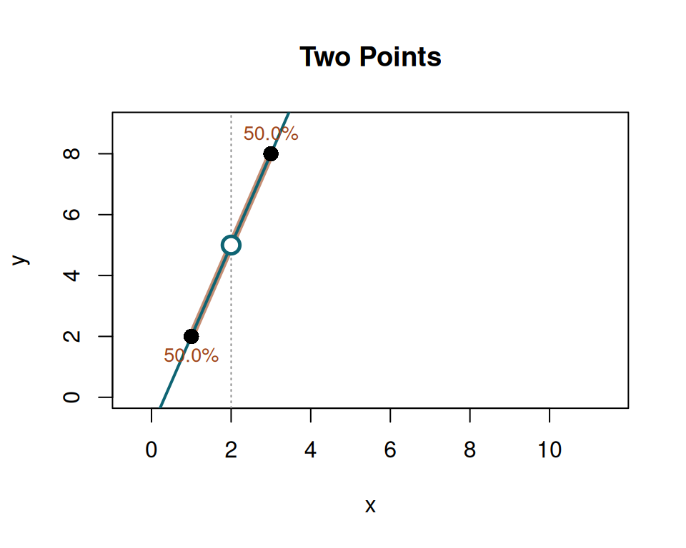
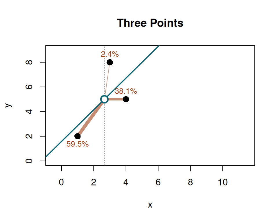
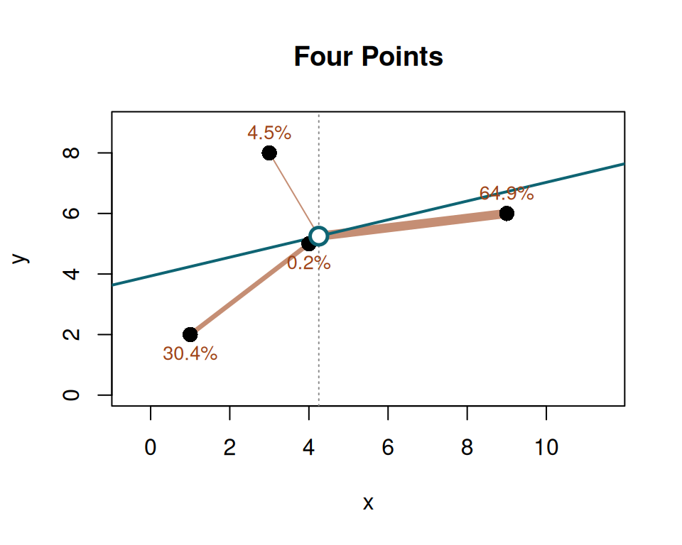
The figures draw the identifying variation $d_i^2$ as the thickness of the ray from the sample centroid $(\bar x, \bar y)$ to each point, with each point's share of the total printed beside it. Squaring concentrates it: a few points far from $\bar x$ can dominate the fit while most points near it contribute almost nothing.
```{r}
#| fig-width: 5
#| fig-height: 4
show <- function(x, y, main = "") {
  xb <- mean(x); yb <- mean(y); d <- x - xb; s <- (y - yb) / d; w <- d^2
  plot(x, y, pch = 16, cex = 1.5, xlim = c(-0.5, 11.5), ylim = c(0, 9),
       xlab = "x", ylab = "y", main = main)
  abline(v = xb, lty = 3, col = "grey55")
  segments(xb, yb, x, y, lwd = 0.6 + 9 * w / sum(w), col = "#9E431899")
  abline(lm(y ~ x), lwd = 2, col = "#0E6473")
  points(x, y, pch = 16, cex = 1.5)
  points(xb, yb, pch = 21, bg = "white", col = "#0E6473", lwd = 2.5, cex = 1.7)
  text(x, y, labels = sprintf("%.1f%%", 100 * w / sum(w)),
       pos = ifelse(y >= yb, 3, 1), cex = .85, col = "#9E4318")
}
show(c(1, 3), c(2, 8), "Two Points")
```
With two points the weights are equal, $50\%$ each.
```{r}
#| fig-width: 5
#| fig-height: 4
show(c(1, 3, 4), c(2, 8, 5), "Three Points")
```
Add a third point at $x=4$ and $\bar x$ moves to $2.67$. The point at $x=3$ now sits almost on top of $\bar x$, so it takes only $2.4\%$ of the weight.
```{r}
#| fig-width: 5
#| fig-height: 4
show(c(1, 3, 4, 9), c(2, 8, 5, 6), "Four Points")
```
Add an extreme point at $x=9$ and $\bar x$ moves to $4.25$. That one observation now carries $65\%$ of the total weight, while $x=4$ falls to $0.18\%$ because it has landed near the new centroid. The weights are relative to the whole sample: add data anywhere and the weights everywhere change.
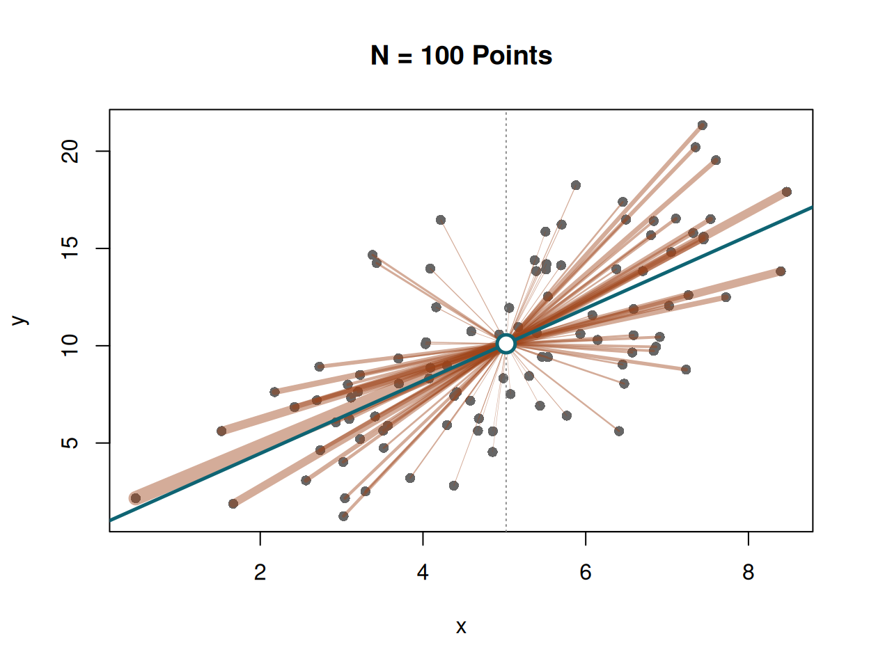
The concentration does not wash out in larger samples. We draw $n = 100$ points, $x_i \sim N(5, 2^2)$ and $y_i = 2 x_i + \varepsilon_i$ with $\varepsilon_i \sim N(0, 3^2)$, and compare the weight held by the ten points nearest $\bar x$ against the ten furthest.
```{r}
#| fig-width: 6.5
#| fig-height: 5
set.seed(3)
n <- 100
x <- rnorm(n, 5, 2)
y <- 2 * x + rnorm(n, 0, 3)

xb <- mean(x); yb <- mean(y); w <- (x - xb)^2
o <- order(w, decreasing = TRUE)

plot(x, y, pch = 16, cex = 1, col = "grey40", xlab = "x", ylab = "y", main = "N = 100 Points")
abline(v = xb, lty = 3, col = "grey55")
segments(xb, yb, x, y, lwd = 0.3 + 10 * w / max(w), col = "#9E431870")
abline(lm(y ~ x), lwd = 2.5, col = "#0E6473")
points(xb, yb, pch = 21, bg = "white", col = "#0E6473", lwd = 2.5, cex = 1.8)
vtab(c(`Weight 10 Nearest Mean (%)`     = 100 * sum(w[o[91:100]]) / sum(w),
        `Weight 10 Furthest (%)`         = 100 * sum(w[o[1:10]]) / sum(w),
        `Effect Weights $d_ix_i < 0$ (%)` = 100 * mean((x - xb) * x < 0),
        `OLS Estimate`                    = coef(lm(y ~ x))[["x"]]), 3)
```
The $10\%$ of points furthest from $\bar x$ hold $35\%$ of the identifying variation; the $10\%$ closest hold $0.14\%$. An observation sitting exactly at $\bar x$ contributes nothing. The last row gives the share of effect weights that are negative: $49\%$, in a sample where no $d_i^2$ can be.
## Binary treatment: OLS weights overlap
Now evaluate $w_i = \tilde V_i V_i$ for a binary treatment with saturated controls. Two readings of the same weights follow: Angrist sorts them by covariate stratum, Słoczyński sorts them by treatment status.
Let $D \in \{0, 1\}$ be a binary treatment and $X$ discrete strata $x \in \{1, \dots, K\}$, with the controls saturated — one indicator per stratum, so no functional form is imposed within cells. Discreteness is essential: saturated controls require a finite number of cells, so continuous $X$ cannot be saturated. With continuous controls the linear projection $\hat D(X)$ is not the cell proportion — it is a linear approximation that can fall outside $[0, 1]$ — and the stratum-by-stratum decomposition below does not go through. With continuous $X$ one could bin it, but the result then holds for the chosen bins, not for $X$ itself.
Residualising $D_i$ on a full set of stratum indicators gives $\tilde D_i = D_i - \hat D(x)$, where $\hat D(x)=n_x^{-1}\sum_{i\in x}D_i$ is the sample treatment fraction in cell $x$. Saturation makes the fitted value equal that cell mean exactly; its population counterpart is the propensity $p(x)=E[D\mid X=x]$. Sum the realised effect weights $w_i = \tilde D_i D_i$ within a stratum:
$$w_x = \sum_{i \in x} \tilde D_i D_i = \sum_{i \in x} D_i^2 - \hat D(x) \sum_{i \in x} D_i = n_x \hat D(x) - n_x \hat D(x)^2 = n_x \hat D(x)(1 - \hat D(x))$$ {#eq-angrist-w}
Nothing new has been added: it is $w_i = \tilde V_i V_i$ from @eq-weff with a binary $V$, where $D_i^2 = D_i$ makes the sum collapse. The maximum at $\hat D(x) = 1/2$ is just the fact that a binary variable has most variance when it is a coin flip.
A single observation with a binary regressor has no slope of its own: forming a difference takes one treated and one control unit. The smallest unit that carries an effect here is the stratum, so what gets weighted is the stratum difference in means.
A word on the labels before going further. $\hat\delta_x$ is a difference in *observed* means within a stratum. Calling the aggregate an ATT or an ATE needs the usual identification conditions: conditional exchangeability, so that treatment is as good as randomly assigned within a stratum, and overlap, so that each stratum holds both treated and control units. Saturation delivers the algebra, not the interpretation. Without those conditions the formulas below still hold exactly, but they describe weighted averages of observed contrasts rather than causal effects. The weighting is what OLS does; whether the thing being weighted is an effect is settled outside the regression.
Let $\hat\delta_x$ be the stratum difference-in-means. Substituting @eq-angrist-w into @eq-weff,
$$\hat\beta_{OLS} = \frac{\sum_{x=1}^K n_x \hat D(x)(1 - \hat D(x))\, \hat\delta_x}{\sum_{x=1}^K n_x \hat D(x)(1 - \hat D(x))}$$ {#eq-angrist}
so strata with propensity near $\hat D(x) = 0.5$ get the most weight per observation. A stratum that contains only treated or only control units has $\hat D(x) = 1$ or $0$, so $w_x = 0$: it drops out entirely, because there is no within-stratum comparison to make. A linear model with continuous controls would extrapolate into those strata instead of dropping them.
## Smaller groups get larger weights
Angrist sorts by covariate stratum. Słoczyński sorts by treatment status instead, collapsing everything into two numbers — the effect on the treated and the effect on the untreated. Aggregating the stratum effects $\hat\delta_x$ of @eq-angrist with each stratum's count of treated or untreated units gives
$$\text{ATT} = \frac{\sum_x n_x \hat D(x)\, \hat\delta_x}{\sum_x n_x \hat D(x)}, \qquad
\text{ATU} = \frac{\sum_x n_x (1 - \hat D(x))\, \hat\delta_x}{\sum_x n_x (1 - \hat D(x))}$$ {#eq-attatu}
and the ATE combines them with their natural shares, $\rho = P(D = 1)$. To see this, write $\text{ATE} = E[\tau_i]$ and condition on treatment status:
$$E[\tau_i] = P(D=1)\, E[\tau_i \mid D=1] + P(D=0)\, E[\tau_i \mid D=0] = \rho\, \text{ATT} + (1 - \rho)\, \text{ATU}.$$
In the finite-sample, stratum-weighted version the same decomposition holds because $\sum_x n_x \hat D(x) = n_1$ and $\sum_x n_x(1-\hat D(x)) = n_0$, so
$$\text{ATE} = \rho\, \text{ATT} + (1 - \rho)\, \text{ATU}$$ {#eq-ate}
The OLS weights of @eq-angrist go as the propensity *variance* $\hat D(x)(1 - \hat D(x))$; the group weights of @eq-attatu go as the propensity itself or its complement. The relation between the two is Słoczyński's result. Write $p = \hat D(X)$ for the cell propensity. Because the design is saturated — the controls are a full set of stratum dummies — residualising $D$ on the strata leaves exactly $\tilde D = D - p$, so the coefficient is $E[\tilde D\, Y]/E[p(1-p)]$. Since $p$ is constant within a stratum, $Y$ enters only through the group means $m_j(p) = E[Y \mid p, D = j]$, and, using $\tilde D = 1 - p$ for treated and $-p$ for untreated units,
$$\beta_{OLS} = \frac{\rho\, E[(1 - p)\, m_1(p) \mid D = 1] - (1 - \rho)\, E[p\, m_0(p) \mid D = 0]}{E[p(1 - p)]}$$ {#eq-sloc1}
Substitute the within-group linear projections $m_j(p) = \alpha_j + \gamma_j p + \varepsilon_j(p)$. The residual term $E[p(1-p)(\varepsilon_1 - \varepsilon_0)]/E[p(1-p)]$ vanishes when the group means are linear in $p$, leaving
$$\beta_{OLS} = (\alpha_1 - \alpha_0) + (\gamma_1 - \gamma_0)\, \frac{E[p^2(1 - p)]}{E[p(1 - p)]}$$ {#eq-sloc2}
The last ratio is moment algebra — an identity in the first three moments of $p$, exact for any distribution. With $\mu_j = E[p \mid D = j]$, $V_j = \text{Var}(p \mid D = j)$, and $w_1, w_0$ the weights defined in @eq-sloc-main below,
$$\frac{E[p^2(1 - p)]}{E[p(1 - p)]} = w_1 \mu_1 + w_0 \mu_0$$ {#eq-moment}
holds identically in the distribution of $p$. Under linearity $\text{ATT} = (\alpha_1 - \alpha_0) + (\gamma_1 - \gamma_0)\mu_1$ and $\text{ATU} = (\alpha_1 - \alpha_0) + (\gamma_1 - \gamma_0)\mu_0$, so @eq-sloc1 through @eq-moment combine into the main result,
$$\hat\beta_{OLS} = w_1\, \text{ATT} + w_0\, \text{ATU}, \qquad
w_1 = \frac{(1 - \rho) V_0}{\rho V_1 + (1 - \rho) V_0}, \quad w_0 = 1 - w_1$$ {#eq-sloc-main}
where $V_j$ is the variance of the propensity score within group $j$. This is exact for the effects of the within-group linear projections; for ATT and ATU it is exact when the group means are linear in $p$ and an approximation otherwise.
Two things about @eq-sloc-main matter. First, the weight $w_1$ on ATT falls as the treated share $\rho$ rises: the larger the treated group, the smaller its say. That is the whole of "smaller groups get more weight," and it does not depend on the propensity variances. Differentiating @eq-sloc-main, $\partial w_1/\partial\rho = -V_0 V_1/(\rho V_1 + (1 - \rho) V_0)^2 < 0$ for any $V_0, V_1 > 0$. The variances set the level of the weight, not the direction it moves. Second, when the propensity has equal variance in the two groups, $V_1 = V_0$, the weights collapse to the reversed shares,
$$\hat\beta_{OLS} \approx (1 - \rho)\, \text{ATT} + \rho\, \text{ATU}$$ {#eq-reversed}
the same two quantities as the ATE in @eq-ate, with the weights **swapped**. At $\rho = 0.1$ the coefficient puts $0.9$ on the effect for the treated tenth; the ATE puts $0.1$ there.
One caveat. @eq-reversed is exact under equal propensity variance across groups — not "no covariates," though no covariates is one trivial way to get there. Słoczyński calls the condition unlikely to hold exactly and offers $\rho$ as a rule of thumb, cleanest near $\rho = 0\%$, $50\%$, or $100\%$.
**Simulation — Angrist and Słoczyński weights.** We draw $n = 400{,}000$ units in five covariate strata ($X \in \{1,\dots,5\}$), each with its own treatment effect $\tau_x = (0, 1, 2, 3, 4)$, so the plain ATE is $2$. The outcome is $y = \tau_x D + X + \varepsilon$. We run the simulation twice with different propensity schedules: once with the treated share near half ($\rho \approx 0.5$, propensities ranging from $0.08$ to $0.93$ across strata) and once with few treated ($\rho \approx 0.09$, propensities from $0.02$ to $0.20$). The point is to show that the OLS coefficient moves with the treated share even though the stratum effects do not change.
```{r}
set.seed(21)
n <- 400000
X <- sample(1:5, n, TRUE)

compare <- function(px) {
  d  <- rbinom(n, 1, px[X]); ta <- c(0, 1, 2, 3, 4)[X]
  yy <- ta * d + X + rnorm(n)
  dt <- resid(lm(d ~ factor(X)))
  nx <- as.vector(table(X)); dh <- as.vector(tapply(d, X, mean))
  DIM <- as.vector(tapply(yy[d == 1], X[d == 1], mean) - tapply(yy[d == 0], X[d == 0], mean))
  rho <- mean(d); ATT <- weighted.mean(ta, d); ATU <- weighted.mean(ta, 1 - d)
  c(`$\\rho$`                    = rho,
    `$\\max\\lvert\\text{weight diff}\\rvert$`         = max(abs(as.vector(tapply(dt * d, X, sum)) - nx*dh*(1-dh))),
    `OLS Saturated`            = unname(coef(lm(yy ~ d + factor(X)))[["d"]]),
    `Angrist Weighted`         = sum(nx*dh*(1-dh) * DIM) / sum(nx*dh*(1-dh)),
    `Sloczynski Approx`        = (1 - rho) * ATT + rho * ATU,
    `ATE`                      = mean(ta))
}
res <- cbind(`$\\rho \\approx 0.5$`  = compare(c(.08, .20, .50, .75, .93)),
             `$\\rho \\approx 0.09$` = compare(c(.02, .04, .08, .12, .20)),
             `$\\rho \\approx 0.91$` = compare(c(.80, .88, .92, .96, .98)))
mtab(res, 4)
```
The two weight vectors — the stratum sums $\sum \tilde D_i D_i$ and Angrist's $n_x \hat D(x)(1 - \hat D(x))$ — are the same, below $10^{-9}$ (the `$\\max\\lvert\\text{weight diff}\\rvert$` row, $0$ to four decimals), and the Angrist-weighted average reproduces the OLS coefficient exactly. With $\rho \approx 0.5$ the coefficient is $2.012$ against an ATE of $1.998$: close, because near-equal shares are where the *grouping by treatment status* does least — the reversed-share gap is $(1 - 2\rho)(\text{ATT} - \text{ATU})$, identically zero at $\rho = 0.5$. That is not a general immunity. The stratum weighting of @eq-angrist survives it, and at any $\rho$ the coefficient still departs from the ATE when the effects line up with $\hat D(x)(1 - \hat D(x))$. Push the treated share to $\rho \approx 0.09$ and the coefficient jumps to $2.874$; push it the other way to $\rho \approx 0.91$ and it falls. The two extremes are symmetric: at $\rho = 0.09$ OLS overweights ATT, at $\rho = 0.91$ it overweights ATU. Nothing about the effects changed. Only the treated share did.
Why does OLS overweight the treated when they are few? The FWL residual is $\tilde D_i = D_i - \hat D(x)$. When $\rho$ is small, $\hat D(x)$ is small in most strata: a treated unit has $\tilde D_i = 1 - \hat D(x) \approx 1$, a control unit has $\tilde D_i = -\hat D(x) \approx 0$. Treated units are the unusual ones — they sit far from the stratum mean of $D$ — so they carry most of the leverage, the same way a point far from $\bar x$ dominates the simple regression. At $\rho = 0.09$ the reversed-share approximation puts weight $1 - \rho = 0.91$ on ATT and only $0.09$ on ATU, while the ATE puts $0.09$ on ATT and $0.91$ on ATU. In observational data where the treated group is small — a common setting — the OLS coefficient can be far from the population average effect even under unconfoundedness, purely because of the weighting.
The reversed-share Słoczyński approximation $(1-\rho)\,\text{ATT} + \rho\,\text{ATU}$ gives $2.029$ against the exact $2.012$, and $2.858$ against $2.874$ — within about a percent, but the exact weights of @eq-sloc-main are what to report.
### The three, side by side
| Decomposition | Sorted by | Smallest effect unit | Exact when | Reference |
|---------------|---------------|---------------|---------------|---------------|
| Observation rule | nothing | the unit effect $\beta_i$ | always | @eq-weff |
| Angrist (1998) | covariate stratum $x$ | stratum difference $\hat\delta_x$ | saturated controls | @eq-angrist |
| Słoczyński (2022) | treatment status $D$ | group averages ATT, ATU | group means linear in $p$; reversed shares also need $V_1 = V_0$ | @eq-reversed |
Read down the last column. The observation rule always holds and says little. Angrist's needs saturation and gives an interpretable weight. Słoczyński's needs more and gives the sharpest statement of the three: the coefficient and the ATE are the same two numbers with the weights reversed. Underneath all of them, Hazlett and Shinkre (2024) show these weights are exactly the bias from fitting a constant effect when effects vary, and argue for estimators that tolerate heterogeneity rather than for diagnosing the weights after the fact.
## Fixed effects: OLS weights movers
In a panel the same rule applies with a different mean subtracted. Unit fixed effects residualise against unit dummies, so $\tilde V_{it} = V_{it} - \bar V_i$, and grouping the observation weights by unit gives that unit's total weight,
$$W_i = \sum_{t=1}^{T} (V_{it} - \bar V_i) V_{it} = \sum_{t=1}^{T} (V_{it} - \bar V_i)^2$$ {#eq-within-square}
its own within sum of squares. So
$$E[\hat\beta_{FE} \mid V, \beta] = \frac{\sum_i W_i \beta_i}{\sum_i W_i}$$ {#eq-fe-target}
A unit whose treatment never changes has $W_i = 0$ and contributes nothing, whatever its effect. Demeaning removes time-invariant confounding; it does not make every unit equally influential.
Pooled OLS drops the dummies, so its deviation is from the grand mean and both channels are in play. Conditioning on the unit and applying the laws of total variance and total covariance splits $\text{Cov}(x,y)$ and $\text{Var}(x)$ each into a within and a between piece, and the pooled slope comes out as a convex combination of the two channel slopes,
$$\text{plim}\;\hat\beta_{OLS} = \frac{V_{within}\, \beta_{within} + V_{between}\, \beta_{between}}{V_{within} + V_{between}}$$ {#eq-pooled}
with $V_{within} = E[\text{Var}(x \mid G)]$, $V_{between} = \text{Var}(E[x \mid G])$, and each $\beta$ the corresponding covariance over variance. Fixed effects removes $V_{between}$ by demeaning and isolates $\beta_{within}$. With two equal groups $V_{between} = \tfrac{1}{4}\Delta\mu^2$, so pulling the group means apart inflates the between weight without touching a single within slope. The [Panel Data Models](panel-data.qmd) chapter develops the decomposition itself.
### Within-unit weighting: an extreme case
A fixed-effects estimate is identified by units whose $x$ changes over time. Units whose $x$ barely moves get near-zero weight regardless of their true effect. So the FE coefficient is a within-variation-weighted average over the units whose $x$ moves, not the population average. When the movers and the stayers have different effects, the two diverge.
The simulation below constructs the extreme version. Half the units barely move and have a true slope of zero; the other half move a lot and have a true slope of two. The average slope across all units is one. The DGP draws $N = 1000$ units for $T = 6$ periods, with $y_{it} = b_i x_{it} + \alpha_i + \varepsilon_{it}$, $\alpha_i \sim N(0,1)$, $\varepsilon_{it} \sim N(0,1)$. Both groups have $E[x_{it}] = 0$, so they differ only in how much $x$ moves within a unit, not in its level.
| Group | Units | $\text{sd}(x_{it})$ | True slope $b_i$ |
|-------|-------|---------------------|-------------------|
| Steady | 1–500 | 0.2 | 0 |
| Movers | 501–1000 | 3 | 2 |
```{r}
set.seed(1)
half <- N / 2
g <- data.frame(id   = rep(1:N, each = T),
                move = rep(c(rep(0.2, half), rep(3, half)), each = T),
                b    = rep(c(rep(0,   half), rep(2, half)), each = T))
g$x <- rnorm(N * T, 0, g$move)
g$y <- g$b * g$x + rep(rnorm(N), each = T) + rnorm(N * T)

wg <- tapply(resid(feols(x ~ 1 | id, g))^2, g$id, sum)
mtab(cbind(value = c(
  `average of the two true slopes`      = mean(c(0, 2)),
  `FE estimate`                         = coef(feols(y ~ x | id, g))[["x"]],
  `Pooled OLS`                          = unname(coef(lm(y ~ x, g))[["x"]]),
  `weight held by the steady half (%)`  = 100 * sum(wg[1:half]) / sum(wg))), 3)
```
Both estimates are near $2$, not the simple average of $1$. The steady units hold under half of one percent of the FE weight: their six observations sit almost on top of their own unit mean, and squaring those tiny deviations puts them nowhere in the sum. Pooled OLS agrees because both groups have $E[x_{it}] = 0$ — there is no between-group difference in $x$ levels, so $V_{between} = 0$ and pooled OLS collapses to $\beta_{within}$. Both estimators weight by variance, and the movers contribute $\sigma^2 = 9$ against the steady group's $0.04$, so neither comes close to the simple average. The two estimators diverge only when the group means of $x$ differ, creating a between channel with its own slope. Shift the steady group's mean $x$ away from zero and the two part company.
### Pulling the groups apart
**Simulation — pulling the groups apart.** The DGP is the same as the within-unit weighting simulation: 500 steady units ($b_i = 0$, $\text{sd}(x) = 0.2$) and 500 movers ($b_i = 2$, $\text{sd}(x) = 3$). The one change is that the steady group's mean $x$ is shifted from $0$ to $10$ or $100$, while the movers stay centred at zero. This opens a gap $\Delta\mu$ between the two group centroids without changing any within-unit slope. The between-slope $\beta_{between} = \Delta\bar y / \Delta\mu$ is near zero, because the steady group's slope is zero and the movers' mean $y$ is also near zero. So as $\Delta\mu$ grows, pooled OLS is dragged toward zero while FE, which removes the between channel by demeaning, stays at $\beta_{within} \approx 2$.
```{r}
b_within <- (0 * 0.2^2 + 2 * 3^2) / (0.2^2 + 3^2)
V_within <- 0.5 * (0.2^2 + 3^2)
predicted <- function(shift) V_within * b_within / (V_within + 0.25 * shift^2)

park <- function(shift) {
  set.seed(1)
  half <- N / 2
  move <- c(rep(0.2, half), rep(3, half))
  b    <- c(rep(0,   half), rep(2, half))
  x    <- rnorm(N * T, 0, rep(move, each = T)) + rep(c(rep(shift, half), rep(0, half)), each = T)
  y    <- rep(b, each = T) * x + rep(rnorm(N), each = T) + rnorm(N * T)
  d    <- data.frame(id = rep(1:N, each = T), x = x, y = y)
  c(`FE estimate`       = coef(feols(y ~ x | id, d))[["x"]],
    `OLS Predicted`     = predicted(shift),
    `OLS Actual`        = coef(lm(y ~ x, d))[["x"]])
}

mtab(t(sapply(c(`shift 0` = 0, `shift 10` = 10, `shift 100` = 100), park)), 3)
```
Fixed effects stays flat near the theoretical $\beta_{within} = 1.991$ wherever the steady group sits. Plain OLS falls from $1.983$ to $0.004$ on identical true slopes: as $\Delta\mu$ grows, the between weight $\tfrac{1}{4}\Delta\mu^2$ swamps the fixed within weight $4.52$, and the coefficient is dragged toward $\beta_{between} = 0$ like $9/(4.52 + \Delta\mu^2/4)$, the numerator $\tfrac{1}{2}(\beta_1 \sigma_1^2 + \beta_2 \sigma_2^2) = 9$.
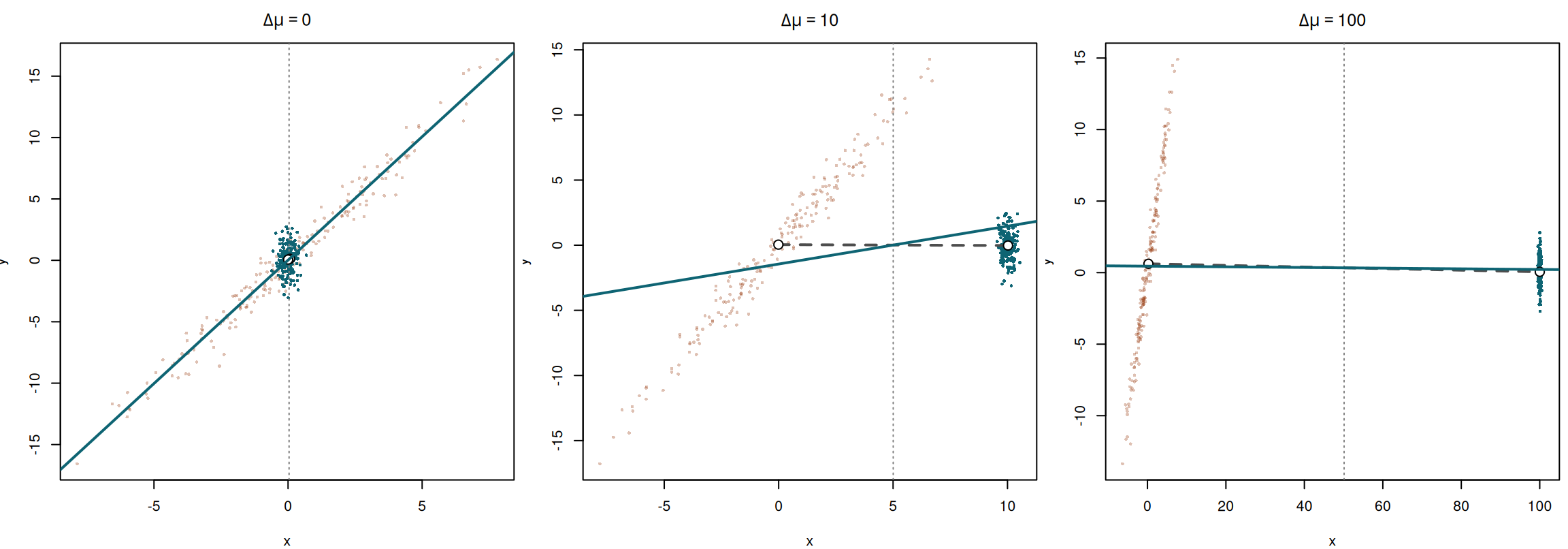
The figure below draws this directly. Two groups of 200 points each share the same within-group slopes: movers have $y = 2x + \varepsilon$ with $x \sim N(0, 3^2)$, the steady group has $y = \varepsilon$ with $x \sim N(\text{shift}, 0.2^2)$. Across the three panels the shift increases from $0$ to $10$ to $100$, opening a gap $\Delta\mu$ between the group centroids without changing any within-group slope. The dashed line connects the two centroids (the between-slope), and the solid line is the pooled OLS fit. As the centroids separate, the between channel dominates and the pooled fit rotates from $\beta_{within} \approx 2$ toward $\beta_{between} \approx 0$.
```{r}
#| fig-width: 12
#| fig-height: 4.2
#| fig-cap: "Pooled OLS as a within/between blend (@eq-pooled). Points are the two groups, open circles their centroids. The dashed line is the between-slope $\\beta_{between} = \\Delta\\bar y/\\Delta\\mu$ through the centroids; the solid line is the pooled fit $\\hat\\beta_{OLS}$. The within slopes are identical across panels; widening $\\Delta\\mu$ (left to right) inflates $V_{between}$ and rotates $\\hat\\beta_{OLS}$ toward $\\beta_{between}$."
set.seed(5)
m <- 200
draw <- function(shift, main) {
  xw <- rnorm(m, 0, 3);       yw <- 2 * xw + rnorm(m)
  xs <- rnorm(m, shift, 0.2); ys <- rnorm(m)
  x <- c(xw, xs); y <- c(yw, ys)
  plot(x, y, pch = 16, cex = .5, col = c(rep("#9E431855", m), rep("#0E6473", m)),
       xlab = "x", ylab = "y", main = main)
  abline(v = mean(x), lty = 3, col = "grey50")
  segments(mean(xw), mean(yw), mean(xs), mean(ys), lty = 2, lwd = 2, col = "grey30")
  points(c(mean(xw), mean(xs)), c(mean(yw), mean(ys)), pch = 21, bg = "white", cex = 1.4)
  abline(lm(y ~ x), lwd = 2, col = "#0E6473")
  dmu <- mean(xs) - mean(xw)
  Vb  <- 0.25 * dmu^2
  Vw  <- 0.5 * (var(xs) + var(xw))
  c(`Within Slope (movers)` = unname(coef(lm(yw ~ xw))[2]),
    `Within Slope (steady)` = unname(coef(lm(ys ~ xs))[2]),
    `Between Slope`      = unname((mean(ys) - mean(yw)) / dmu),
    `Between Weight (%)` = 100 * Vb / (Vb + Vw),
    `OLS Estimate`       = unname(coef(lm(y ~ x))[2]))
}
op <- par(mfrow = c(1, 3), mar = c(4, 3.5, 2.5, 0.5))
a <- draw(0,   expression(Delta*mu == 0))
b <- draw(10,  expression(Delta*mu == 10))
c_ <- draw(100, expression(Delta*mu == 100))
par(op)
mtab(cbind(`$\\Delta\\mu = 0$` = a, `$\\Delta\\mu = 10$` = b, `$\\Delta\\mu = 100$` = c_), 3)
```
Read across the three columns. The within slopes barely change — about $2$ for the movers, indistinguishable from zero for the steady strip. What changes is the between weight: $0.03\%$ when the centres coincide, $85\%$ at $\Delta\mu = 10$, and $99.6\%$ at $\Delta\mu = 100$. So the OLS fit falls from $2.01$ to $0.29$ to $0.02$ on identical true slopes.
The between slope reported in the first column is meaningless — and harmlessly so: with the centres nearly on top of each other $\Delta\mu \approx 0$, an unstable ratio is multiplied by a vanishing weight and contributes nothing.
The strip has influence in the second and third panels despite barely moving. Influence is distance from the mean of $x$, and the strip sits $\Delta\mu$ units from it; what it contributes is not its slope but its position — it anchors one end of the dashed line.
A group dummy removes that channel. Demeaning subtracts each cloud's *own* mean, sliding the shifted strip back to the centre, so every panel collapses onto the first — centroids coinciding. Run OLS on that and the solid fit swings back up to the within slope. That is all fixed effects is, and why its slope matches the leftmost panel's regardless of how far the strip had been pushed.
So "the weight is how much $x$ moves" is the demeaned case only. It is exact once unit effects are removed, and false in general, because with the halves at different levels of $x$ part of the fitted line is a comparison *between* them rather than a weighting of within-unit slopes.
## When does the weighting change the answer?
The variance-weighted average equals the plain average whenever effects are unrelated to the weights. The weighting tilts the estimate only when units whose $x$ moves more have systematically different slopes — that is, when $b_i$ covaries with $w_i$.
The gap is exactly a covariance. For any weights $w_i$,
$$\frac{\sum_i w_i \beta_i}{\sum_i w_i} - \bar\beta = \frac{\text{Cov}_n(w_i, \beta_i)}{\bar w}$$ {#eq-weight-gap}
If high-effect units carry more weight the coefficient exceeds the plain average; if they carry less it falls below; if weights and effects are unrelated the gap is zero. Nothing about the estimator is broken in any of the three cases.
The following two designs illustrate the distinction. Both draw $N = 1000$ units, $T = 6$ periods, with $\text{sd}_i(x) \sim U(0.2, 3)$ and $y_{it} = b_i x_{it} + \alpha_i + \varepsilon_{it}$. Both share the same $x$. What differs is how the true slopes $b_i$ relate to regressor volatility:
- **(A) Unrelated:** $b_i \sim N(1, 1)$, independent of $\text{sd}_i(x)$.
- **(B) Aligned:** $b_i = 1 + 0.8(\text{sd}_i - 1.6)$, so the slope rises with volatility.
Both designs average to $\bar b \approx 1$. The question is whether the FE estimate — a variance-weighted average of the $b_i$ — differs from that plain average.
```{r}
set.seed(7)
sdX <- runif(N, 0.2, 3)

panel <- function(b) {
  h   <- data.frame(id = rep(1:N, each = T),
                    x  = rnorm(N * T, 0, rep(sdX, each = T)))
  h$y <- rep(b, each = T) * h$x + rep(rnorm(N), each = T) + rnorm(N * T)
  h
}
compareAB <- function(h, b) {
  w <- tapply(resid(feols(x ~ 1 | id, h))^2, h$id, sum)
  c(`FE estimate`            = coef(feols(y ~ x | id, h))[["x"]],
    `true slopes, plain avg` = mean(b),
    `true slopes, weighted`  = sum(w * b) / sum(w))
}

b1 <- rnorm(N, 1, 1)
b2 <- 1 + 0.8 * (sdX - 1.6)
h1 <- panel(b1); h2 <- panel(b2)

mtab(cbind(`(A) unrelated` = compareAB(h1, b1),
            `(B) aligned`   = compareAB(h2, b2)), 4)
```
In (A) all three numbers agree to within sampling noise: the weighting is there but costs nothing, because the slopes are independent of the weights. In (B) the FE estimate is $1.53$ while the plain average of the true slopes is $1.01$, and the weighted average, $1.54$, confirms what the estimator was tracking all along — it overweights the high-slope units precisely because they are the high-variance units.
FE still removes confounding from the unit effects $\alpha_i$ — that is its job, and it does it in both designs. What FE does not do is change the within-variance weighting. Even after demeaning, OLS leans on units whose $x$ moves more, and in design (B) those units happen to have higher slopes. The gap between the FE estimate and the plain average is not a failure of FE; it is what OLS does by construction, and it matters only when $b_i$ covaries with $\text{Var}_i(x)$. Without knowing the true slopes, the problem is undetectable from the data alone — the FE estimate looks well-behaved, standard errors are fine, it is just consistently estimating a different parameter than the simple average.
**Reweighting to recover the simple average.** One response is weighted least squares. The FE weight on unit $i$ is proportional to its within-variance $\hat\sigma_i^2 = \sum_t (x_{it} - \bar x_i)^2$. In this model, running WLS-FE with weight $1/\hat\sigma_i^2$ gives each unit equal influence, so the estimate targets the simple average of slopes rather than the variance-weighted average. This is the logic behind Gibbons, Suárez Serrato, and Urbancic (2018), who formalize the reweighting to recover what they call the "unit-average treatment effect," and it is the continuous analog of Słoczyński's reweighting in the binary case.
The trade-off is efficiency. The high-variance units are the ones whose slope is best estimated — their $x$ moves a lot, so there is real information there. Downweighting them inflates the standard error. We are giving up precision to change which parameter we estimate.
The weights are also not always available. A unit whose $x$ never moves has $\hat\sigma_i^2 = 0$, so its weight is undefined, and a unit that barely moves gets an explosive one. A panel with true stayers forces a choice — drop them or bound the weights — and either choice changes the population the estimate refers to. Inverse-within-variation weighting swaps a variation-weighted target for a unit-weighted one; whether that is the right swap depends on the estimand, not on the weighting being more neutral.
The table below adds the reweighted FE estimate to both designs.
```{r}
compareAB2 <- function(h, b) {
  wvar <- tapply(resid(feols(x ~ 1 | id, h))^2, h$id, sum)
  inv_w <- 1 / tapply(resid(feols(x ~ 1 | id, h))^2, h$id, mean)
  h$rw <- rep(inv_w, each = T)
  c(`FE estimate`            = coef(feols(y ~ x | id, h))[["x"]],
    `Reweighted FE`          = coef(feols(y ~ x | id, h, weights = ~rw))[["x"]],
    `true slopes, plain avg` = mean(b),
    `true slopes, weighted`  = sum(wvar * b) / sum(wvar))
}

mtab(cbind(`(A) unrelated` = compareAB2(h1, b1),
            `(B) aligned`   = compareAB2(h2, b2)), 4)
```
In (A) the reweighted estimate agrees with the standard FE estimate — reweighting changes nothing when effects are independent of variance. In (B) the reweighted estimate falls from $1.53$ back to near $1.01$, recovering the simple average. The price is a larger standard error, because we have deliberately downweighted the most informative units.
Standard errors do not reveal any of this. An estimate can be precise, and unbiased for its own weighted target, while answering a different question from the one that was asked. The issue is the estimand, not estimator failure.
## Start with the estimand
Before interpreting an OLS coefficient, ask which average effect is the substantive target: the average across people, the average among the treated, the average across firms, the effect where there is overlap. Then compare that target with the weights the specification implies.
If the two differ, the response depends on the application. Report the weighted estimand for what it is, model the heterogeneity, or reweight toward the population of interest. Reweighting is not free — observations with little residual variation carry little information, so giving them more influence costs precision, as the reweighted fixed-effects estimate above shows.
The lesson is not to avoid OLS. It is to stop calling the coefficient "the average effect" without checking which average the regression built.
## Summary
1. **One rule.** OLS weights each observation by $w_i = \tilde V_i V_i$, the regressor times what is left of it after the controls (@eq-weff). The weights sum to $\sum_i \tilde V_i^2 \ge 0$; individual weights need not be positive.
2. **Cross-section.** With binary treatment and saturated strata the weight on a stratum is $n_x \hat D(x)(1 - \hat D(x))$ (@eq-angrist): overlap gets the weight, and a stratum with no comparison gets none. Sorted by treatment status instead, the same weights put $1 - \rho$ on the ATT and $\rho$ on the ATU (@eq-reversed) — the ATE's own shares, reversed.
3. **Panel.** Under fixed effects a unit's weight is its own within sum of squares (@eq-within-square): movers are the estimate, stayers are not. Drop the dummies and group-mean differences re-enter through $V_{between}\beta_{between}$ (@eq-pooled).
4. **When it matters.** The weighting always happens. It moves the answer only when the effects line up with the weights, and then by exactly $\text{Cov}_n(w_i, \beta_i)/\bar w$ (@eq-weight-gap).
Everything here is the *effect* reading — weights on the unobservable $\beta_i$, answering what $\hat\beta$ estimates. The same FWL identity also weights the *observed* outcomes, a signed and fully computable combination that answers which rows drive the number and reaches, unchanged, into estimators far beyond OLS. That is the companion chapter, [Interpreting OLS: Outcome Weights](outcome-weights.qmd).