4 Weights in OLS in causal inference

Published

January 16, 2025

4.1 Unit level weights for OLS

This chapter follows Chad Hazlett and Tanvi Shinkre (2024), “Demystifying and avoiding the OLS ‘weighting problem’: unmodeled heterogeneity and straightforward solutions,” arXiv:2403.03299.

Under unconfoundedness, the identifying assumption holds at each level of $X$. When $X$ is discrete and low-dimensional, we can stratify and compute the ATE by the g-formula. In practice we usually run a linear regression

\[ Y = \alpha + \beta D + \gamma X + \epsilon \tag{4.1}\]

and treat $\hat\beta$ as the treatment effect, relying on linearity to span the covariate space. The question is what this estimator is actually weighting.

Suppose we are interested in the ATE of $D$ on $Y$. Say we have discrete variables $X$. Under unconfoundedness, the ATE is

\[ \begin{aligned} \tau_{ATE} &= \sum E[Y(1) - Y(0) | X = x] P(X = x) \\ &= \sum (E[Y|D=1, X=x]- E[Y|D=0, X=x]) P(X=x) \\ &= \sum DIM_x P(X=x) \\ \end{aligned} \tag{4.2}\]

This is basically the g-formula, or regression adjustment formula. We compute the DIM (difference in means) between treated and control for each strata $X=x$, then the weighted average is the ATE, with $\hat P(X=x)$ as weights.

If we have high dimensional $X$, we usually do \[ Y = \beta_0 + \beta_1 X + \delta_{reg} D + \epsilon \tag{4.3}\]

We would hope $\delta_{reg}$ is close to $\delta_{ATE}$, but we are not sure.

OLS coefficients are:

\[ \hat \beta = (Z'Z)^{-1} Z'y \tag{4.4}\]

Here I use $Z$ to represent all regressors. Each coefficient is a weighted sum of the outcome,

\[ \hat \tau_{reg} = \sum \omega_i Y_i \tag{4.5}\]

By FWL theorem,

\[ \hat \tau_{reg} = \frac{\sum Y_i (D_i - \hat d(X_i)) }{\sum (D_i - \hat d(X_i))^2} \tag{4.6}\]

Here $\hat d(X_i) = \hat p(D_i=1|X_i)$ which is the predicted value of linear regression of $D$ on $X$. The numerator is the covariance between $Y$ and residualized $D$, the denominator is the variance of the residualized $D$. Note that the original FWL would have residualized $Y$ here, but it turns out it works the same with the original $Y$.

Therefore the weights are

\[ \begin{aligned} \omega_i &= \frac{D_i - \hat d(X_i)}{\sum (D_i - \hat d(X_i))^2} \\ \end{aligned} \tag{4.7}\]

Note for the denominator, it’s a constant. It does not scale the weights to sum to one — they sum to zero, because $D_i - \hat d(X_i)$ is an OLS residual from a regression that includes an intercept. What the denominator normalizes is the contrast: since $\sum D_i(D_i - \hat d(X_i)) = \sum (D_i - \hat d(X_i))^2$ (the residual is orthogonal to the fitted values), we get $\sum_i \omega_i D_i = 1$, i.e. the weights on the treated sum to $+1$ and those on the control sum to $-1$. That is what makes $\sum_i \omega_i Y_i$ a weighted difference of means. The numerator for treated units are $1-\hat d(X_i)$, for control units it’s $-\hat d(X_i)$ (negative). It is similar to IPW weights, which are $1/\hat d(X_i)$ for treated and $1/(1-\hat d(X_i))$ for control. These two sets of weights go the same direction. For the treated, the higher probability of being treated, the lower weight; for the control, the higher probability of being treated, the larger the magnitude of the (negative) weight.

If these weights are the same as the IPW weights, then we’ll get $\tau_{reg}=\tau_{ATE}$. However, they are usually different.

Another way to write this as weighted difference in means:

\[ \hat \tau_{wdim} = \sum \omega_i Y_i = \sum_{i:D=1} \tilde \omega_i Y_i + \sum_{i:D=0} \tilde \omega_i Y_i \tag{4.8}\]

where, with $c = \sum (D_i - \hat d(X_i))^2$, the per-arm weights are $\tilde \omega_i = (1-\hat d(X_i))/c$ for treated units ($D_i=1$) and $\tilde \omega_i = -\hat d(X_i)/c$ for control units ($D_i=0$)

Because $\hat d(X_i)$ is from a linear probability model, it’s possible that it’s not between 0 and 1. In that case, we can have negative weights. The negative weights could mean the observations do not have a match in the other group. For example, $\hat d(X_i) > 1$ will cause the weight $(1-\hat d(X_i))/c$ to flip sign and become negative for a treated unit. That means this unit is more like treated units than any control units. In other words, there is no match in the control group. The mirror image happens for a control unit with $\hat d(X_i) < 0$: its weight $-\hat d(X_i)/c$ flips to positive, so it enters the contrast on the same side as the treated. Either way the unit contributes with the wrong sign.

The negative weights are invisible unless we examine $\hat d(X_i)$ directly — which is to say, unless we look at the propensity score. A linear regression of $Y$ on $D$ and $X$ hides the extrapolation. So $\hat\tau_{\text{reg}}$ is a weighted average of outcomes with weights that differ from the ATE weights, and some of those weights may carry the wrong sign without the researcher knowing.

4.2 Strata level weights

Angrist (1998, Econometrica) has the strata-wise weights for OLS:

\[ \hat \tau_{reg} = \frac{\sum_x \hat \tau_x \hat d(x) (1-\hat d(x)) \hat P(X=x)}{\sum_x \hat d(x) (1-\hat d(x)) \hat P(X=x)} \tag{4.9}\]

this shows that different from ATE, these weights are $\hat d(x) (1-\hat d(x)) \hat P(X=x)$. The stratas are weighted not only by $P(X_i=x)$, but also by the variance of treatment status. When $\hat d(X_i)$ is close to .5, the weight is the largest.

If there is no treatment effect heterogeneity, then it does not matter how you weight. When there is treatment effect heterogeneity, this estimator could be very different from ATE.

Hazlett and Shinkre show that Angrist’s formula is a special case: it is exact when the probability of treatment is linear in $X$ (as in a saturated model with discrete $X$). They derive a more general formula, but the Angrist version suffices under linearity of $d(X)$.

4.3 Recommended estimation approaches

Under constant effects and linearity, $E[Y \mid X, D] = \beta_0 + \beta_1 X + \beta_2 D$, a regression of $Y$ on $D$ and $X$ recovers the ATE without further adjustment. When the linearity or constant-effects assumption fails, Hazlett and Shinkre suggest relaxing to separate linearity — allowing different intercepts for $Y(0)$ and $Y(1)$. Under that weaker assumption, several estimators are unbiased for the ATE.

The interaction (Lin 2013) estimator regresses $Y$ on $D$, $\tilde X = X - \bar X$, and $D \tilde X$; the coefficient on $D$ is the ATE. The imputation estimator fits separate regressions for treated and control, predicts counterfactual outcomes for the other group, and takes the average difference — algebraically, it returns the same estimate. Stratification and g-computation do the same for discrete $X$: compute the stratum-level difference in means and weight by the stratum probability.

All of these still rely on linearity within each arm. When that fails, matching (e.g. mean-balancing) or nonparametric estimation is needed.

4.4 A worked example

We make the regression weights $\omega_i$ concrete and compare them to IPW weights $1/\hat d(X_i)$ (treated) and $1/(1-\hat d(X_i))$ (control).

We draw $n = 500$ observations with a single covariate $X \sim N(0,1)$, treatment $D \sim \text{Bernoulli}(\Lambda(0.5X))$ — so 238 units are treated — and outcome $Y = 1 + 2D + 1.5X + \varepsilon$ with $\varepsilon \sim N(0,1)$. The effect is constant at 2, so there is no heterogeneity for the weights to mis-average; the point of this first example is only to show that the weights reproduce the coefficient.

Code

library(dplyr)

set.seed(1)
n <- 500
X <- rnorm(n)
d_prob <- plogis(0.5 * X)
D <- rbinom(n, 1, d_prob)
Y <- 1 + 2 * D + 1.5 * X + rnorm(n)
dat <- data.frame(Y, D, X)

# Regression-implied weights via the FWL residualization of D on X.
d_hat <- fitted(lm(D ~ X, data = dat))
resid_D <- dat$D - d_hat
omega_reg <- resid_D / sum(resid_D^2)

# IPW weights (Horvitz-Thompson), using the same linear-probability d_hat
# purely for comparability with the regression weights above.
ipw <- ifelse(dat$D == 1, 1 / d_hat, 1 / (1 - d_hat))
# rescale by a single constant so the treated weights average 1; this only
# fixes the axis scale of the plot below and does not change any comparison
ipw <- ipw / sum(ipw[dat$D == 1]) * sum(dat$D == 1)

tau_reg <- sum(omega_reg * dat$Y)
tau_lm  <- coef(lm(Y ~ D + X, data = dat))["D"]

data.frame(tau_reg_from_weights = tau_reg, tau_from_lm_coef = tau_lm)

  tau_reg_from_weights tau_from_lm_coef
D             2.084644         2.084644

Both give 2.084644, identical to seven digits, confirming $\hat\tau_{reg} = \sum \omega_i Y_i$. (Both sit a little above the true 2; with $n=500$ and a constant effect that is sampling noise, not weighting.)

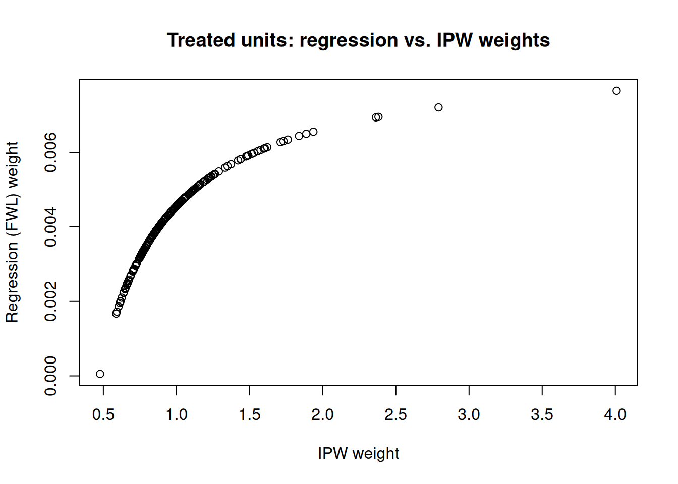
Plotting omega_reg against ipw for treated and control units separately shows the two weighting schemes move in the same direction but are not proportional.

Be careful about what that does and does not establish. Non-proportional weights are necessary for $\hat\tau_{reg}$ to differ from the ATE, not sufficient. In this example the effect is constant at 2, so every unit’s effect is the same number and any weights that form a difference of means return that number: $\hat\tau_{reg}$ and the ATE coincide here no matter how oddly the weights are distributed. A weighting problem needs two ingredients, and this design has only one. The section after next supplies the other.

Code

par(mfrow = c(1, 2))
plot(ipw[dat$D == 1], omega_reg[dat$D == 1],
     xlab = "IPW weight", ylab = "Regression (FWL) weight",
     main = "Treated units")
plot(ipw[dat$D == 0], omega_reg[dat$D == 0],
     xlab = "IPW weight", ylab = "Regression (FWL) weight",
     main = "Control units")

Code

par(mfrow = c(1, 1))

Both panels slope upward and neither is a straight line through the origin: the two schemes rank units the same way but do not scale together, which is the whole content of $\hat\tau_{reg} \neq \hat\tau_{ATE}$.

Note also what this example does not show. Here $\hat d(X_i)$ stays inside $[0.062, 0.994]$, so every weight keeps its expected sign and the negative-weight problem discussed above never materializes. That is a property of this particular design, not a reassurance. We now strengthen the selection from $\Lambda(0.5X)$ to $\Lambda(3X)$, holding everything else fixed, and the linear probability model starts predicting outside the unit interval:

Code

set.seed(2)
X2 <- rnorm(n)
D2 <- rbinom(n, 1, plogis(3 * X2))       # much stronger selection on X
dat2 <- data.frame(D = D2, X = X2)
d_hat2 <- fitted(lm(D ~ X, data = dat2))
omega2 <- (dat2$D - d_hat2) / sum((dat2$D - d_hat2)^2)

data.frame(
  dhat_below_0        = sum(d_hat2 < 0),
  dhat_above_1        = sum(d_hat2 > 1),
  treated_wrong_sign  = sum(dat2$D == 1 & omega2 < 0),
  control_wrong_sign  = sum(dat2$D == 0 & omega2 > 0)
)

  dhat_below_0 dhat_above_1 treated_wrong_sign control_wrong_sign
1           28           42                 42                 28

The fitted probabilities now run from $-0.367$ to $1.445$. Twenty-eight units fall below zero and 42 rise above one, and the wrong-sign counts match those two numbers exactly: 42 treated units carry a negative weight and 28 control units carry a positive one. That is not a coincidence but the mechanism described above — every unit with $\hat d > 1$ here is treated, every unit with $\hat d < 0$ is control, and each flips the sign of its own contribution. In total 70 of 500 observations, 14% of the sample, enter the contrast on the wrong side.

Those units are the ones with no counterpart in the other arm, and a plain regression of $Y$ on $D$ and $X$ gives you no indication that they are there. Nothing in the coefficient table changes appearance; only looking at $\hat d(X_i)$ reveals it.

This is a property of the regression weights specifically, and the reason is worth being explicit about. $\hat d(X_i)$ here is not a propensity score we chose to estimate with a linear probability model; it is the object OLS implicitly uses, because the FWL residualisation of $D$ on $X$ is a linear regression. Linear fitted values are not confined to $[0,1]$, so out-of-range values, and with them wrong-sign weights, are always available to OLS. Genuine IPW weights built from a logit or probit propensity score cannot do this: $\hat\pi(X)$ lies strictly inside $(0,1)$ by construction, so $1/\hat\pi$ and $1/(1-\hat\pi)$ stay positive. IPW has its own failure mode when $\hat\pi$ approaches 0 or 1 — weights explode, and the estimate rests on a handful of observations — but it is a visible one. The ipw vector plotted above is deliberately built from the same linear $\hat d$ so that the two weighting schemes are comparable unit by unit; it is a diagnostic device, not the IPW estimator one would actually run.

4.5 When the weights actually bite

Neither example so far has shown $\hat\tau_{reg}$ miss the ATE, because neither had heterogeneous effects. This one does, and it is built on discrete $X$ so that every quantity in this chapter can be computed exactly rather than approximated.

Let $X \in \{0, 1, 2\}$ with probabilities $0.4, 0.3, 0.3$; let the treatment probability be $d(x) = 0.5, 0.1, 0.9$; and let the effect be $\tau(x) = 1, 4, 4$. The outcome is $Y = 1 + \tau(X)D + 2X + \varepsilon$ with $\varepsilon \sim N(0,1)$, and we draw $n = 20{,}000$. The design is chosen so that the stratum where treatment is most balanced, $x = 0$ with $d = 0.5$, is also the stratum with the small effect.

The population ATE follows from the definition: $0.4(1) + 0.3(4) + 0.3(4) = 2.8$. Angrist’s strata-level formula above weights each stratum by $d(x)\{1-d(x)\}P(X=x)$ instead — that is $0.10, 0.027, 0.027$, or $0.649, 0.175, 0.175$ once normalised, against the true shares $0.4, 0.3, 0.3$. The $x=0$ stratum carries 65% of the regression’s weight and 40% of the ATE’s, so the regression should be pulled toward that stratum’s effect of 1.

Code

set.seed(11)
n  <- 20000
px <- c(0.4, 0.3, 0.3)          # P(X = 0, 1, 2)
dx <- c(0.5, 0.1, 0.9)          # P(D = 1 | X)
tx <- c(1,   4,   4)            # tau(X)

X   <- sample(0:2, n, TRUE, prob = px)
D   <- rbinom(n, 1, dx[X + 1])
Y   <- 1 + tx[X + 1] * D + 2 * X + rnorm(n)
dat3 <- data.frame(Y, D, X = factor(X))

# What OLS returns
tau_ols <- coef(lm(Y ~ D + X, data = dat3))["D"]

# Angrist's variance-weighted average of the stratum effects, computed from the
# population quantities rather than estimated
w   <- dx * (1 - dx) * px
ang <- sum(w * tx) / sum(w)

# g-computation on a saturated arm-specific model
m   <- lm(Y ~ D * X, data = dat3)
tau_g <- mean(predict(m, transform(dat3, D = 1)) -
              predict(m, transform(dat3, D = 0)))

# Lin's interaction estimator: D, centred covariates, and their interaction
Xc  <- scale(model.matrix(~ X, dat3)[, -1, drop = FALSE], scale = FALSE)
tau_lin <- coef(lm(dat3$Y ~ dat3$D + Xc + dat3$D:Xc))[2]

data.frame(population_ATE = sum(px * tx),
           angrist_formula = ang,
           ols_coefficient = tau_ols,
           g_computation = tau_g,
           lin_interaction = tau_lin, row.names = NULL)

  population_ATE angrist_formula ols_coefficient g_computation lin_interaction
1            2.8        2.051948        2.082158      2.839965        2.839965

The OLS coefficient is 2.08 against a population ATE of 2.80. It is not a noisy estimate of the ATE; it is a precise estimate of something else. Angrist’s formula predicts 2.052 from the population quantities alone, and the regression delivers 2.082 — the gap between those two is sampling noise, while the gap between either of them and 2.80 is the weighting problem. The regression is answering a question about the stratum where treatment happens to be most balanced, and nothing in its output says so.

The two recommended estimators recover the ATE, and recover it identically: g-computation and Lin’s interaction estimator both return 2.840, against a realised sample ATE of 2.814. That they agree to every printed digit is the algebraic equivalence noted in the previous section, not a coincidence of this draw. Both work here because the saturated model in a discrete $X$ satisfies separate linearity exactly — each arm’s conditional mean is linear in the stratum dummies, since it is saturated in them.

The practical reading is that the weighting problem needs heterogeneity and non-proportional weights together. The first two examples had the weights; this one adds the heterogeneity, and the cost appears immediately. Since one rarely knows in advance whether effects are heterogeneous, the cheap insurance is to run the interaction or imputation estimator by default: under constant effects it returns what OLS would have returned, and under heterogeneity it returns the ATE that OLS would have missed.

--- title: "Weights in OLS in causal inference" date: "2025-01-16" --- ## Unit level weights for OLS This chapter follows Chad Hazlett and Tanvi Shinkre ([2024](https://arxiv.org/abs/2403.03299)), “Demystifying and avoiding the OLS ‘weighting problem’: unmodeled heterogeneity and straightforward solutions,” arXiv:2403.03299. Under unconfoundedness, the identifying assumption holds at each level of $X$. When $X$ is discrete and low-dimensional, we can stratify and compute the ATE by the g-formula. In practice we usually run a linear regression $$ Y = \alpha + \beta D + \gamma X + \epsilon $$ {#eq-weights-ols-1} and treat $\hat\beta$ as the treatment effect, relying on linearity to span the covariate space. The question is what this estimator is actually weighting. Suppose we are interested in the ATE of $D$ on $Y$. Say we have discrete variables $X$. Under unconfoundedness, the ATE is $$ \begin{aligned} \tau_{ATE} &= \sum E[Y(1) - Y(0) | X = x] P(X = x) \\ &= \sum (E[Y|D=1, X=x]- E[Y|D=0, X=x]) P(X=x) \\ &= \sum DIM_x P(X=x) \\ \end{aligned} $$ {#eq-weights-ols-2} This is basically the g-formula, or regression adjustment formula. We compute the DIM (difference in means) between treated and control for each strata $X=x$, then the weighted average is the ATE, with $\hat P(X=x)$ as weights. If we have high dimensional $X$, we usually do $$ Y = \beta_0 + \beta_1 X + \delta_{reg} D + \epsilon $$ {#eq-weights-ols-3} We would hope $\delta_{reg}$ is close to $\delta_{ATE}$, but we are not sure. OLS coefficients are: $$ \hat \beta = (Z'Z)^{-1} Z'y $$ {#eq-weights-ols-4} Here I use $Z$ to represent all regressors. Each coefficient is a weighted sum of the outcome, $$ \hat \tau_{reg} = \sum \omega_i Y_i $$ {#eq-weights-ols-5} By FWL theorem, $$ \hat \tau_{reg} = \frac{\sum Y_i (D_i - \hat d(X_i)) }{\sum (D_i - \hat d(X_i))^2} $$ {#eq-weights-ols-6} Here $\hat d(X_i) = \hat p(D_i=1|X_i)$ which is the predicted value of linear regression of $D$ on $X$. The numerator is the covariance between $Y$ and residualized $D$, the denominator is the variance of the residualized $D$. Note that the original FWL would have residualized $Y$ here, but it turns out it works the same with the original $Y$. Therefore the weights are $$ \begin{aligned} \omega_i &= \frac{D_i - \hat d(X_i)}{\sum (D_i - \hat d(X_i))^2} \\ \end{aligned} $$ {#eq-weights-ols-7} Note for the denominator, it's a constant. It does *not* scale the weights to sum to one --- they sum to **zero**, because $D_i - \hat d(X_i)$ is an OLS residual from a regression that includes an intercept. What the denominator normalizes is the contrast: since $\sum D_i(D_i - \hat d(X_i)) = \sum (D_i - \hat d(X_i))^2$ (the residual is orthogonal to the fitted values), we get $\sum_i \omega_i D_i = 1$, i.e. the weights on the treated sum to $+1$ and those on the control sum to $-1$. That is what makes $\sum_i \omega_i Y_i$ a weighted *difference* of means. The numerator for treated units are $1-\hat d(X_i)$, for control units it's $-\hat d(X_i)$ (negative). It is similar to IPW weights, which are $1/\hat d(X_i)$ for treated and $1/(1-\hat d(X_i))$ for control. These two sets of weights go the same direction. For the treated, the higher probability of being treated, the lower weight; for the control, the higher probability of being treated, the larger the magnitude of the (negative) weight. If these weights are the same as the IPW weights, then we'll get $\tau_{reg}=\tau_{ATE}$. However, they are usually different. Another way to write this as weighted difference in means: $$ \hat \tau_{wdim} = \sum \omega_i Y_i = \sum_{i:D=1} \tilde \omega_i Y_i + \sum_{i:D=0} \tilde \omega_i Y_i $$ {#eq-weights-ols-8} where, with $c = \sum (D_i - \hat d(X_i))^2$, the per-arm weights are $\tilde \omega_i = (1-\hat d(X_i))/c$ for treated units ($D_i=1$) and $\tilde \omega_i = -\hat d(X_i)/c$ for control units ($D_i=0$) Because $\hat d(X_i)$ is from a linear probability model, it's possible that it's not between 0 and 1. In that case, we can have negative weights. The negative weights could mean the observations do not have a match in the other group. For example, $\hat d(X_i) > 1$ will cause the weight $(1-\hat d(X_i))/c$ to flip sign and become negative for a treated unit. That means this unit is more like treated units than any control units. In other words, there is no match in the control group. The mirror image happens for a control unit with $\hat d(X_i) < 0$: its weight $-\hat d(X_i)/c$ flips to *positive*, so it enters the contrast on the same side as the treated. Either way the unit contributes with the wrong sign. The negative weights are invisible unless we examine $\hat d(X_i)$ directly — which is to say, unless we look at the propensity score. A linear regression of $Y$ on $D$ and $X$ hides the extrapolation. So $\hat\tau_{\text{reg}}$ is a weighted average of outcomes with weights that differ from the ATE weights, and some of those weights may carry the wrong sign without the researcher knowing. ## Strata level weights Angrist ([1998](https://doi.org/10.2307/2999578), *Econometrica*) has the strata-wise weights for OLS: $$ \hat \tau_{reg} = \frac{\sum_x \hat \tau_x \hat d(x) (1-\hat d(x)) \hat P(X=x)}{\sum_x \hat d(x) (1-\hat d(x)) \hat P(X=x)} $$ {#eq-weights-ols-9} this shows that different from ATE, these weights are $\hat d(x) (1-\hat d(x)) \hat P(X=x)$. The stratas are weighted not only by $P(X_i=x)$, but also by the variance of treatment status. When $\hat d(X_i)$ is close to .5, the weight is the largest. If there is no treatment effect heterogeneity, then it does not matter how you weight. When there is treatment effect heterogeneity, this estimator could be very different from ATE. Hazlett and Shinkre show that Angrist's formula is a special case: it is exact when the probability of treatment is linear in $X$ (as in a saturated model with discrete $X$). They derive a more general formula, but the Angrist version suffices under linearity of $d(X)$. ## Recommended estimation approaches Under constant effects and linearity, $E[Y \mid X, D] = \beta_0 + \beta_1 X + \beta_2 D$, a regression of $Y$ on $D$ and $X$ recovers the ATE without further adjustment. When the linearity or constant-effects assumption fails, Hazlett and Shinkre suggest relaxing to *separate* linearity — allowing different intercepts for $Y(0)$ and $Y(1)$. Under that weaker assumption, several estimators are unbiased for the ATE. The interaction (Lin [2013](https://doi.org/10.1214/12-AOAS583)) estimator regresses $Y$ on $D$, $\tilde X = X - \bar X$, and $D \tilde X$; the coefficient on $D$ is the ATE. The imputation estimator fits separate regressions for treated and control, predicts counterfactual outcomes for the other group, and takes the average difference — algebraically, it returns the same estimate. Stratification and g-computation do the same for discrete $X$: compute the stratum-level difference in means and weight by the stratum probability. All of these still rely on linearity within each arm. When that fails, matching (e.g. mean-balancing) or nonparametric estimation is needed. ## A worked example We make the regression weights $\omega_i$ concrete and compare them to IPW weights $1/\hat d(X_i)$ (treated) and $1/(1-\hat d(X_i))$ (control). We draw $n = 500$ observations with a single covariate $X \sim N(0,1)$, treatment $D \sim \text{Bernoulli}(\Lambda(0.5X))$ — so 238 units are treated — and outcome $Y = 1 + 2D + 1.5X + \varepsilon$ with $\varepsilon \sim N(0,1)$. The effect is constant at 2, so there is no heterogeneity for the weights to mis-average; the point of this first example is only to show that the weights reproduce the coefficient. ```{r} #| label: fwl-weights-example #| cache: true #| warning: false #| message: false library(dplyr) set.seed(1) n <- 500 X <- rnorm(n) d_prob <- plogis(0.5 * X) D <- rbinom(n, 1, d_prob) Y <- 1 + 2 * D + 1.5 * X + rnorm(n) dat <- data.frame(Y, D, X) # Regression-implied weights via the FWL residualization of D on X. d_hat <- fitted(lm(D ~ X, data = dat)) resid_D <- dat$D - d_hat omega_reg <- resid_D / sum(resid_D^2) # IPW weights (Horvitz-Thompson), using the same linear-probability d_hat # purely for comparability with the regression weights above. ipw <- ifelse(dat$D == 1, 1 / d_hat, 1 / (1 - d_hat)) # rescale by a single constant so the treated weights average 1; this only # fixes the axis scale of the plot below and does not change any comparison ipw <- ipw / sum(ipw[dat$D == 1]) * sum(dat$D == 1) tau_reg <- sum(omega_reg * dat$Y) tau_lm <- coef(lm(Y ~ D + X, data = dat))["D"] data.frame(tau_reg_from_weights = tau_reg, tau_from_lm_coef = tau_lm) ``` Both give 2.084644, identical to seven digits, confirming $\hat\tau_{reg} = \sum \omega_i Y_i$. (Both sit a little above the true 2; with $n=500$ and a constant effect that is sampling noise, not weighting.) Plotting `omega_reg` against `ipw` for treated and control units separately shows the two weighting schemes move in the same direction but are not proportional. Be careful about what that does and does not establish. Non-proportional weights are *necessary* for $\hat\tau_{reg}$ to differ from the ATE, not sufficient. In this example the effect is constant at 2, so every unit's effect is the same number and any weights that form a difference of means return that number: $\hat\tau_{reg}$ and the ATE coincide here no matter how oddly the weights are distributed. A weighting problem needs two ingredients, and this design has only one. The section after next supplies the other. ```{r} #| label: fwl-weights-plot #| cache: true #| warning: false #| message: false par(mfrow = c(1, 2)) plot(ipw[dat$D == 1], omega_reg[dat$D == 1], xlab = "IPW weight", ylab = "Regression (FWL) weight", main = "Treated units") plot(ipw[dat$D == 0], omega_reg[dat$D == 0], xlab = "IPW weight", ylab = "Regression (FWL) weight", main = "Control units") par(mfrow = c(1, 1)) ``` Both panels slope upward and neither is a straight line through the origin: the two schemes rank units the same way but do not scale together, which is the whole content of $\hat\tau_{reg} \neq \hat\tau_{ATE}$. Note also what this example does *not* show. Here $\hat d(X_i)$ stays inside $[0.062, 0.994]$, so every weight keeps its expected sign and the negative-weight problem discussed above never materializes. That is a property of this particular design, not a reassurance. We now strengthen the selection from $\Lambda(0.5X)$ to $\Lambda(3X)$, holding everything else fixed, and the linear probability model starts predicting outside the unit interval: ```{r} #| label: fwl-negative-weights #| cache: true #| warning: false #| message: false set.seed(2) X2 <- rnorm(n) D2 <- rbinom(n, 1, plogis(3 * X2)) # much stronger selection on X dat2 <- data.frame(D = D2, X = X2) d_hat2 <- fitted(lm(D ~ X, data = dat2)) omega2 <- (dat2$D - d_hat2) / sum((dat2$D - d_hat2)^2) data.frame( dhat_below_0 = sum(d_hat2 < 0), dhat_above_1 = sum(d_hat2 > 1), treated_wrong_sign = sum(dat2$D == 1 & omega2 < 0), control_wrong_sign = sum(dat2$D == 0 & omega2 > 0) ) ``` The fitted probabilities now run from $-0.367$ to $1.445$. Twenty-eight units fall below zero and 42 rise above one, and the wrong-sign counts match those two numbers exactly: 42 treated units carry a negative weight and 28 control units carry a positive one. That is not a coincidence but the mechanism described above — every unit with $\hat d > 1$ here is treated, every unit with $\hat d < 0$ is control, and each flips the sign of its own contribution. In total 70 of 500 observations, 14% of the sample, enter the contrast on the wrong side. Those units are the ones with no counterpart in the other arm, and a plain regression of $Y$ on $D$ and $X$ gives you no indication that they are there. Nothing in the coefficient table changes appearance; only looking at $\hat d(X_i)$ reveals it. This is a property of the *regression* weights specifically, and the reason is worth being explicit about. $\hat d(X_i)$ here is not a propensity score we chose to estimate with a linear probability model; it is the object OLS implicitly uses, because the FWL residualisation of $D$ on $X$ *is* a linear regression. Linear fitted values are not confined to $[0,1]$, so out-of-range values, and with them wrong-sign weights, are always available to OLS. Genuine IPW weights built from a logit or probit propensity score cannot do this: $\hat\pi(X)$ lies strictly inside $(0,1)$ by construction, so $1/\hat\pi$ and $1/(1-\hat\pi)$ stay positive. IPW has its own failure mode when $\hat\pi$ approaches 0 or 1 — weights explode, and the estimate rests on a handful of observations — but it is a visible one. The `ipw` vector plotted above is deliberately built from the same linear $\hat d$ so that the two weighting schemes are comparable unit by unit; it is a diagnostic device, not the IPW estimator one would actually run. ## When the weights actually bite Neither example so far has shown $\hat\tau_{reg}$ miss the ATE, because neither had heterogeneous effects. This one does, and it is built on discrete $X$ so that every quantity in this chapter can be computed exactly rather than approximated. Let $X \in \{0, 1, 2\}$ with probabilities $0.4, 0.3, 0.3$; let the treatment probability be $d(x) = 0.5, 0.1, 0.9$; and let the effect be $\tau(x) = 1, 4, 4$. The outcome is $Y = 1 + \tau(X)D + 2X + \varepsilon$ with $\varepsilon \sim N(0,1)$, and we draw $n = 20{,}000$. The design is chosen so that the stratum where treatment is most balanced, $x = 0$ with $d = 0.5$, is also the stratum with the small effect. The population ATE follows from the definition: $0.4(1) + 0.3(4) + 0.3(4) = 2.8$. Angrist's strata-level formula above weights each stratum by $d(x)\{1-d(x)\}P(X=x)$ instead — that is $0.10, 0.027, 0.027$, or $0.649, 0.175, 0.175$ once normalised, against the true shares $0.4, 0.3, 0.3$. The $x=0$ stratum carries 65% of the regression's weight and 40% of the ATE's, so the regression should be pulled toward that stratum's effect of 1. ```{r} #| label: weighting-bites #| cache: true #| warning: false #| message: false set.seed(11) n <- 20000 px <- c(0.4, 0.3, 0.3) # P(X = 0, 1, 2) dx <- c(0.5, 0.1, 0.9) # P(D = 1 | X) tx <- c(1, 4, 4) # tau(X) X <- sample(0:2, n, TRUE, prob = px) D <- rbinom(n, 1, dx[X + 1]) Y <- 1 + tx[X + 1] * D + 2 * X + rnorm(n) dat3 <- data.frame(Y, D, X = factor(X)) # What OLS returns tau_ols <- coef(lm(Y ~ D + X, data = dat3))["D"] # Angrist's variance-weighted average of the stratum effects, computed from the # population quantities rather than estimated w <- dx * (1 - dx) * px ang <- sum(w * tx) / sum(w) # g-computation on a saturated arm-specific model m <- lm(Y ~ D * X, data = dat3) tau_g <- mean(predict(m, transform(dat3, D = 1)) - predict(m, transform(dat3, D = 0))) # Lin's interaction estimator: D, centred covariates, and their interaction Xc <- scale(model.matrix(~ X, dat3)[, -1, drop = FALSE], scale = FALSE) tau_lin <- coef(lm(dat3$Y ~ dat3$D + Xc + dat3$D:Xc))[2] data.frame(population_ATE = sum(px * tx), angrist_formula = ang, ols_coefficient = tau_ols, g_computation = tau_g, lin_interaction = tau_lin, row.names = NULL) ``` The OLS coefficient is 2.08 against a population ATE of 2.80. It is not a noisy estimate of the ATE; it is a precise estimate of something else. Angrist's formula predicts 2.052 from the population quantities alone, and the regression delivers 2.082 — the gap between those two is sampling noise, while the gap between either of them and 2.80 is the weighting problem. The regression is answering a question about the stratum where treatment happens to be most balanced, and nothing in its output says so. The two recommended estimators recover the ATE, and recover it identically: g-computation and Lin's interaction estimator both return 2.840, against a realised sample ATE of 2.814. That they agree to every printed digit is the algebraic equivalence noted in the previous section, not a coincidence of this draw. Both work here because the saturated model in a discrete $X$ satisfies separate linearity exactly — each arm's conditional mean is linear in the stratum dummies, since it is *saturated* in them. The practical reading is that the weighting problem needs heterogeneity and non-proportional weights together. The first two examples had the weights; this one adds the heterogeneity, and the cost appears immediately. Since one rarely knows in advance whether effects are heterogeneous, the cheap insurance is to run the interaction or imputation estimator by default: under constant effects it returns what OLS would have returned, and under heterogeneity it returns the ATE that OLS would have missed.