---
title: "Causal Forest in panel data"
date: "2017-10-23"
---
## Introduction
In this simulation exercise, we use Causal Forest (Now is implemented in Generalized Random Forest) (https://github.com/swager/grf) to calculated conditional average treatment effect (or heterogeneous treatment effect). We assume three different data generating processes. The first one is a linear interaction between a variable of interest and the treatment dummy. The second one assumes a nonlinear function (a step function) of a variable of interest, say $X$, and the treatment dummy $W$. The third one is also nonlinear, assuming we have variable $X$, but the real DGP is the interaction of log of $X$ and $W$.
## Linear effect
Suppose we have a panel of firms over time, treatment assignment is random. We split the data into training and test. Then we generate 10 random variables, the first two are highly correlated. Then we collapse V2 into firm means, and use that as the unit effect. That is, we have a DGP as:
$$y_{it} = \alpha_i + V1_{it} + W_{it} + V1_{it}*W_{it} + \epsilon_{it} $$
Here $\alpha_i$ is not observed, and it is correlated with $V1$. If we don't control for it, we are going to have a biased estimator.
We run a fixed effect model, and a random effect model and an OLS model. We expect fixed effect model will do well, but not the other two. This is because the other two models do not control for $\alpha_i$ directly.
```{r}
#| label: chunk1
#| warning: false
#| cache: true
#| message: false
# This is a simulation exercise to see how causal forest performs
# First we run a linear model, with panel setting
# Then two nonlinear situations, with panel setting.

library(lfe, quietly = TRUE)
library(lme4)
require(snowfall)
library(MASS)
library(grf)
library(tidyverse)
set.seed(666)
rm(list = ls())
# t is no. of periods. p is no. of variables, n is no. of firms.
t <- 10
p <- 10
n=400
# generate p random variables
data1 = as.data.frame(matrix(rnorm(n*t*p), n*t, p))
names(data1) <- paste0("X", 1:p)

firm=seq(1,n)
time=seq(1,t)
data <- expand.grid(firm=firm,time=time)


# W is the treatment assignment
data$W <- rbinom(n*t, 1, 0.5)
data$train <- rbinom(n*t, 1, 0.5)


# generate two correlated variables
covarMat = matrix( c(1, .95^2, .95^2, 1 ) , nrow=2 , ncol=2 )
data.2  = as.data.frame(mvrnorm(n=n*t , mu=rep(0,2), Sigma=covarMat ))
names(data.2) <- c("V1", "V2")

data <- bind_cols(data,data.2) %>%
    tibble()

data <- bind_cols(data,data1)

# generate unit effect by firm means of V2, which is correlated with V1
data <- data %>%
    group_by(firm) %>%
    mutate(unit.effect=mean(V2)) %>%
    ungroup() %>%
    arrange(firm, time)

y<-c()
unit<-c()
X<-c()
k <- 0
for(i in 1:n){
    for(j in 1:t){
        k<-k+1
        unit[k]<-i
        y[k]<-1+ data$V1[k] + data$W[k] + data$V1[k]*data$W[k] + data$unit.effect[k]+rnorm(1,mean=0,sd=1)
    }
}
data$unit=unit
data$y=y


data.train <- data %>%
    filter(train==1)
data.test <- data %>%
    filter(train==0)

# run fixed effect, random effect, and ols to see whether they are
# biased.
# in general we should expect fe performs better, since we are
# omitting unit.effect in the other two models
fe <- felm(y ~ V1 * W | unit, data=data.train)
re <-lmer(y~V1*W+(1 | unit), data=data.train)
ols <- lm(y ~ V1 * W , data=data.train)
summary(fe)
summary(re)
summary(ols)
```
Now we run Causal Forest on this data. Two clarifications about what is and is not at stake here. First, treatment $W$ is **randomized** (`rbinom(., 0.5)`, independent of the firm effect), so the omitted unit effect $\alpha_i$ does *not* confound the treatment effect — it only enters the nuisance functions (and hence precision), it does not create treatment-effect bias. The panel issue here is therefore mainly *dependence and nuisance fit*, not confounding. Second, the firm structure should be handled in two ways: we include the firm dummies in $X$ so the forest can absorb $\alpha_i$ in the nuisance models, **and** we pass `clusters = firm` so that `grf`'s honest sample splitting and its variance estimates keep each firm's repeated observations together rather than treating them as independent rows. Including the dummies alone does neither of those.
```{r}
#| label: chunk2
#| warning: false
#| cache: true
#| message: false
# ensure consistent factor levels across train/test
all_firms <- levels(factor(data$firm))
data.train$firm <- factor(data.train$firm, levels = all_firms)
data.test$firm <- factor(data.test$firm, levels = all_firms)

# a is a data set of firm dummies
# Caution: this one-hot-encodes all ~400 firms into individual dummy columns
# of X. Random forests split poorly on such a high-cardinality sparse block
# of binary columns (each dummy is only informative for a tiny fraction of
# observations). A fixed-effects forest (demean y, W, and the continuous
# covariates within firm first, then run causal_forest on the demeaned
# variables) or a method that handles unit effects natively would typically
# perform better than including firm as raw dummies.
a <- as.data.frame(model.matrix(y~firm, data.train))
X <- as.matrix(bind_cols(data.train[,c(5,7:16)],a))
Y <- data.train$y
W <- data.train$W
# causal forest is run on y against V1, to X10 and firm dummies.
# clusters = firm makes honest splitting and the variance estimates respect
# the panel structure (a firm's repeated rows are kept together, not treated
# as independent observations).
tau.forest = causal_forest(X, Y, W, clusters = as.integer(data.train$firm))

average_treatment_effect(tau.forest, target.sample = "all")
average_treatment_effect(tau.forest, target.sample = "treated")
a <- as.data.frame(model.matrix(y~firm, data.test))
X.test <- as.matrix(bind_cols(data.test[,c(5,7:16)],a))
Y.test <- data.test$y
W.test <- data.test$W

tau.hat = predict(tau.forest, X.test, estimate.variance = TRUE)
sigma.hat = sqrt(tau.hat$variance.estimates)

data.test$pred <- tau.hat$predictions
ggplot(data.test, aes(x=V1, y=pred)) + geom_point() + geom_abline(intercept = 1, slope = 1)
```
This graph is the predicted value of CATE on the test data, vs. the value of $V1$.
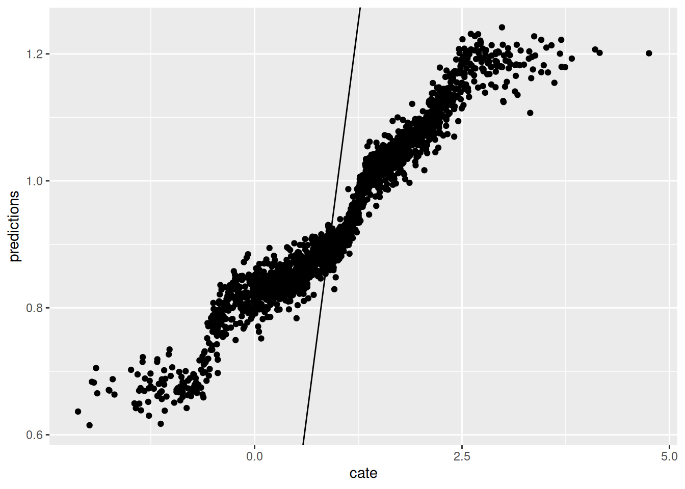
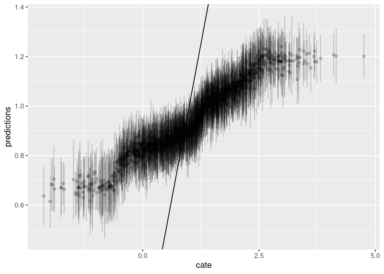
Now we graph the predicted CATE against the true CATE. The other nice feature of Causal Forest is that it returns variance for CATE for each observation. We also graph the error bar here.
```{r}
#| label: chunk3
#| warning: false
#| cache: true
#| message: false
graph.data  <- as.data.frame(tau.hat )
graph.data  <- graph.data  %>%
    mutate(cate=1+data.test$V1) %>%
    mutate(lower=predictions - sigma.hat , upper=predictions + sigma.hat )

ggplot(graph.data , aes(x=cate, y=predictions)) + geom_point()  + geom_abline(slope = 1)
ggplot() + geom_errorbar(graph.data , mapping=aes(x=cate, ymin=lower,ymax=upper), alpha = 0.2) + geom_point(graph.data , mapping=aes(x=cate, y=predictions), alpha = 0.2) + geom_abline(slope = 1)
```
## Nonlinear effect case 1
In the first situation, we assume DGP:
$$y_{it} = 1 + \alpha_i + max(V1_{it},0)*W_{it} + \epsilon_{it} $$
```{r}
#| label: chunk4
#| warning: false
#| cache: true
#| message: false
# if we have a nonlinear effect
# suppose we have the same X, but y is generated nonlinearly.
# in this example, y is a nonlinear function of V1 and W
set.seed(666)
rm(list = ls())
# t is no. of periods. p is no. of variables, n is no. of firms.
t <- 10
p <- 10
n=400
# generate p random variables
data1 = as.data.frame(matrix(rnorm(n*t*p), n*t, p))
names(data1) <- paste0("X", 1:p)

firm=seq(1,n)
time=seq(1,t)
data <- expand.grid(firm=firm,time=time)


# W is the treatment assignment
data$W <- rbinom(n*t, 1, 0.5)
data$train <- rbinom(n*t, 1, 0.5)


# generate two correlated variables
covarMat = matrix( c(1, .95^2, .95^2, 1 ) , nrow=2 , ncol=2 )
data.2  = as.data.frame(mvrnorm(n=n*t , mu=rep(0,2), Sigma=covarMat ))
names(data.2) <- c("V1", "V2")

data <- bind_cols(data,data.2) %>%
    tibble()

data <- bind_cols(data,data1)

# generate unit effect by firm means of V2, which is correlated with V1
data <- data %>%
    group_by(firm) %>%
    mutate(unit.effect=mean(V2)) %>%
    ungroup() %>%
    arrange(firm, time)

y<-c()
unit<-c()
X<-c()
k <- 0
for(i in 1:n){
    for(j in 1:t){
        k<-k+1
        unit[k]<-i
        y[k]<-1+ pmax(data$V1[k],0)*data$W[k]  + data$unit.effect[k]+rnorm(1,mean=0,sd=1)
    }
}
data$y=y
data$unit <- unit

data.train <- data %>%
    filter(train==1)
data.test <- data %>%
    filter(train==0)

# run fixed effect, random effect, and ols to see whether they are
# biased.
# they all perform poorly
fe <- felm(y ~ V1 * W | unit, data=data.train)
re <-lmer(y~V1*W+(1 | unit), data=data.train)
ols <- lm(y ~ V1 * W , data=data.train)
summary(fe)
summary(re)
summary(ols)
```
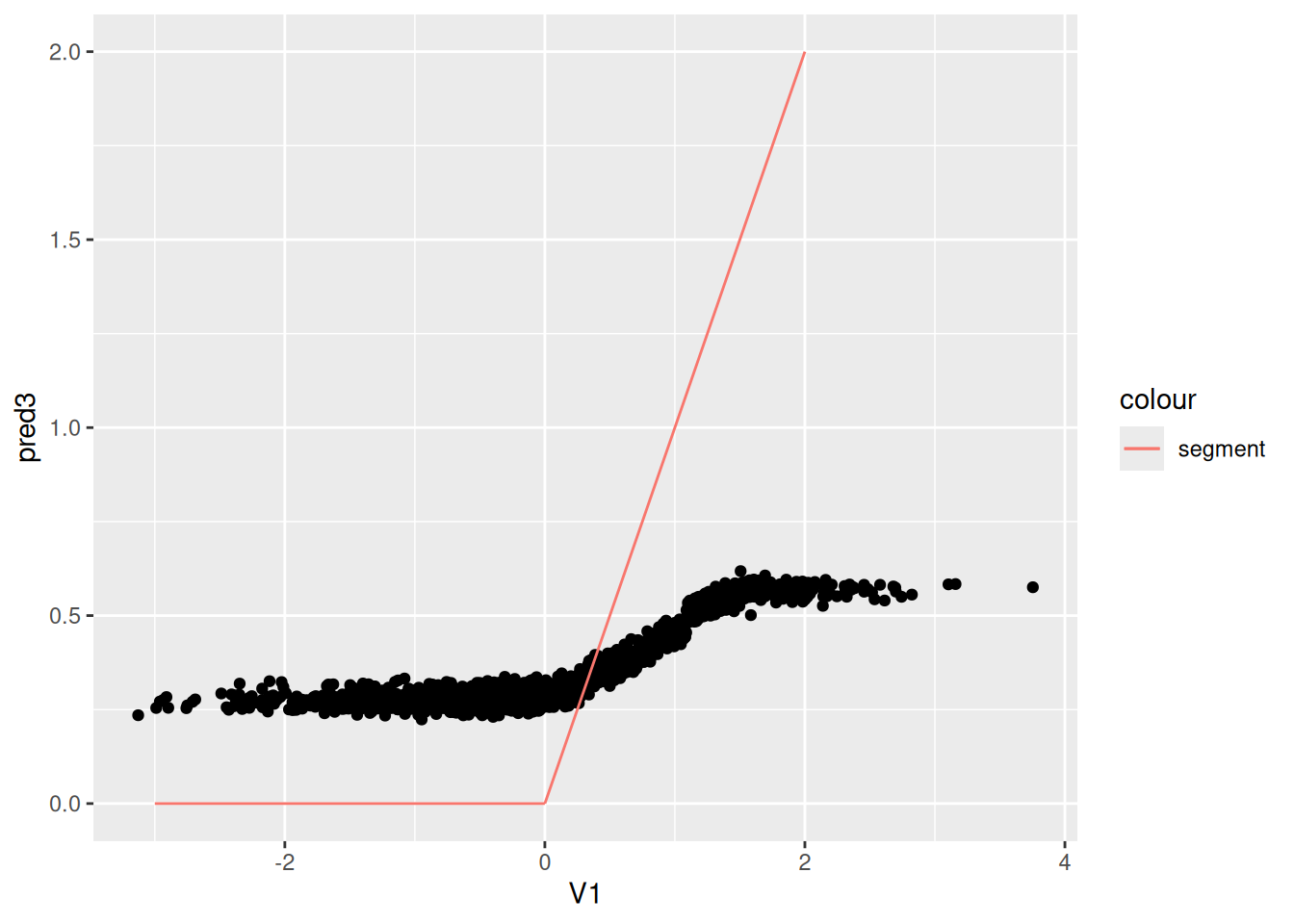
Apparently none of these model will return anything meaningful.
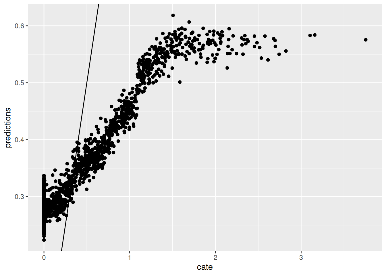
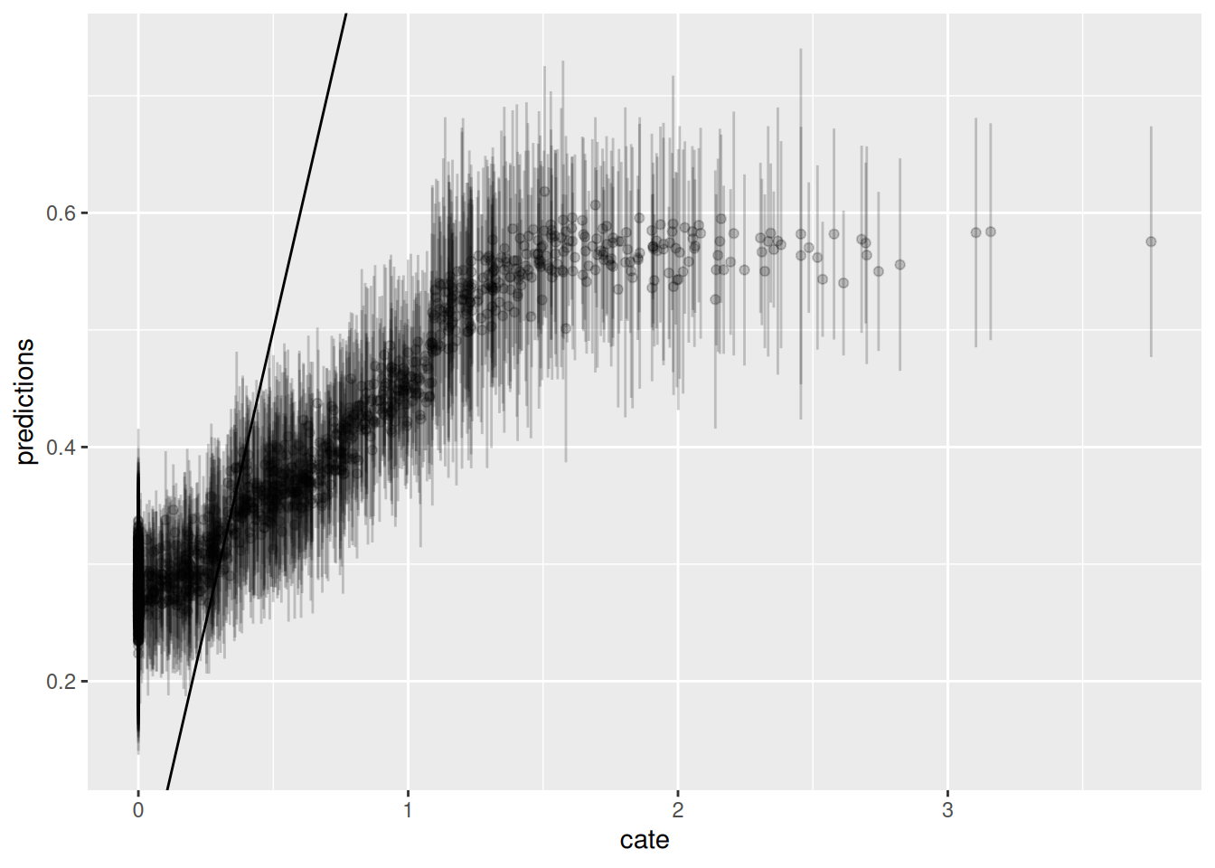
Now we use Causal Forest. The first graph is the predicted CATE against $V1$; the second graph is the predicted CATE against true CATE. The third one adds in error bars.
```{r}
#| label: chunk5
#| warning: false
#| cache: true
#| message: false
all_firms <- levels(factor(data$firm))
data.train$firm <- factor(data.train$firm, levels = all_firms)
data.test$firm <- factor(data.test$firm, levels = all_firms)

# a is a data set of firm dummies
a <- as.data.frame(model.matrix(y~firm,data.train))
X <- as.matrix(bind_cols(data.train[,c(5,7:16)],a))
Y <- data.train$y
W <- data.train$W

#tau.forest = causal_forest(X, Y, W, num.trees = 4000)
a <- as.data.frame(model.matrix(y~firm,data.test))
X.test <- as.matrix(bind_cols(data.test[,c(5,7:16)],a))
Y.test <- data.test$y
W.test <- data.test$W

tau.forest3 = causal_forest(X, Y, W, clusters = as.integer(data.train$firm))

average_treatment_effect(tau.forest3, target.sample = "all")
average_treatment_effect(tau.forest3, target.sample = "treated")
#tau.forest3 = causal_forest(X, Y, W, num.trees = 4000)
tau.hat3 = predict(tau.forest3, X.test, estimate.variance = TRUE)
sigma.hat3 = sqrt(tau.hat3$variance.estimates)

data.test$pred3 <- tau.hat3$predictions

seg1 <- data.frame(x1 = -3, x2 = 0, y1 = 0, y2 = 0)
seg2 <- data.frame(x1 = 0, x2 = 2, y1 = 0, y2 = 2)
ggplot(data.test, aes(x=V1, y=pred3)) + geom_point() +
geom_segment(aes(x = x1, y = y1, xend = x2, yend = y2, colour = "segment"), data = seg1)+
geom_segment(aes(x = x1, y = y1, xend = x2, yend = y2, colour = "segment"), data = seg2)
graph.data3 <- as.data.frame(tau.hat3)
graph.data3 <- graph.data3 %>%
    mutate(cate=pmax(data.test$V1,0)) %>%
    mutate(lower=predictions - sigma.hat3, upper=predictions + sigma.hat3)

ggplot(graph.data3, aes(x=cate, y=predictions)) + geom_point()  + geom_abline(slope = 1)
ggplot() + geom_errorbar(graph.data3, mapping=aes(x=cate, ymin=lower,ymax=upper), alpha = 0.2) + geom_point(graph.data3, mapping=aes(x=cate, y=predictions), alpha = 0.2) + geom_abline(slope = 1)
```
## Nonlinear effect case 2
In the second situation, we assume DGP:
$$y_{it} = 1 + \alpha_i + log(V1_{it}^2)*W_{it} + \epsilon_{it} $$
But we only observe $V1$, not the log of the squared $V1$.
```{r}
#| label: chunk6
#| warning: false
#| cache: true
#| message: false
# if we have a nonlinear effect
# suppose we have the same X, but y is generated nonlinearly.
# another example, suppose we observe log(V1), but the true effect is V1
set.seed(666)
rm(list = ls())
# t is no. of periods. p is no. of variables, n is no. of firms.
t <- 10
p <- 10
n=400
# generate p random variables
data1 = as.data.frame(matrix(rnorm(n*t*p), n*t, p))
names(data1) <- paste0("X", 1:p)

firm=seq(1,n)
time=seq(1,t)
data <- expand.grid(firm=firm,time=time)


# W is the treatment assignment
data$W <- rbinom(n*t, 1, 0.5)
data$train <- rbinom(n*t, 1, 0.5)


# generate two correlated variables
covarMat = matrix( c(1, .95^2, .95^2, 1 ) , nrow=2 , ncol=2 )
data.2  = as.data.frame(mvrnorm(n=n*t , mu=rep(0,2), Sigma=covarMat ))
names(data.2) <- c("V1", "V2")

data <- bind_cols(data,data.2) %>%
    tibble()

data <- bind_cols(data,data1)

# generate unit effect by firm means of V2, which is correlated with V1
data <- data %>%
    group_by(firm) %>%
    mutate(unit.effect=mean(V2)) %>%
    ungroup() %>%
    arrange(firm, time)

y<-c()
unit<-c()
X<-c()
k <- 0
for(i in 1:n){
    for(j in 1:t){
        k<-k+1
        unit[k]<-i
        y[k]<-1+ log(data$V1[k]^2)*data$W[k] + pmin(data$X3[k], 0) + data$unit.effect[k]+rnorm(1,mean=0,sd=1)
    }
}
data$y=y
data$unit <- unit

data.train <- data %>%
    filter(train==1)
data.test <- data %>%
    filter(train==0)

# run fixed effect, random effect, and ols to see whether they are
# biased.
# they all perform poorly
fe <- felm(y ~ V1 * W | unit, data=data.train)
re <-lmer(y~V1*W+(1 | unit), data=data.train)
ols <- lm(y ~ V1 * W , data=data.train)
summary(fe)
summary(re)
summary(ols)
```
Again, these models do not work.
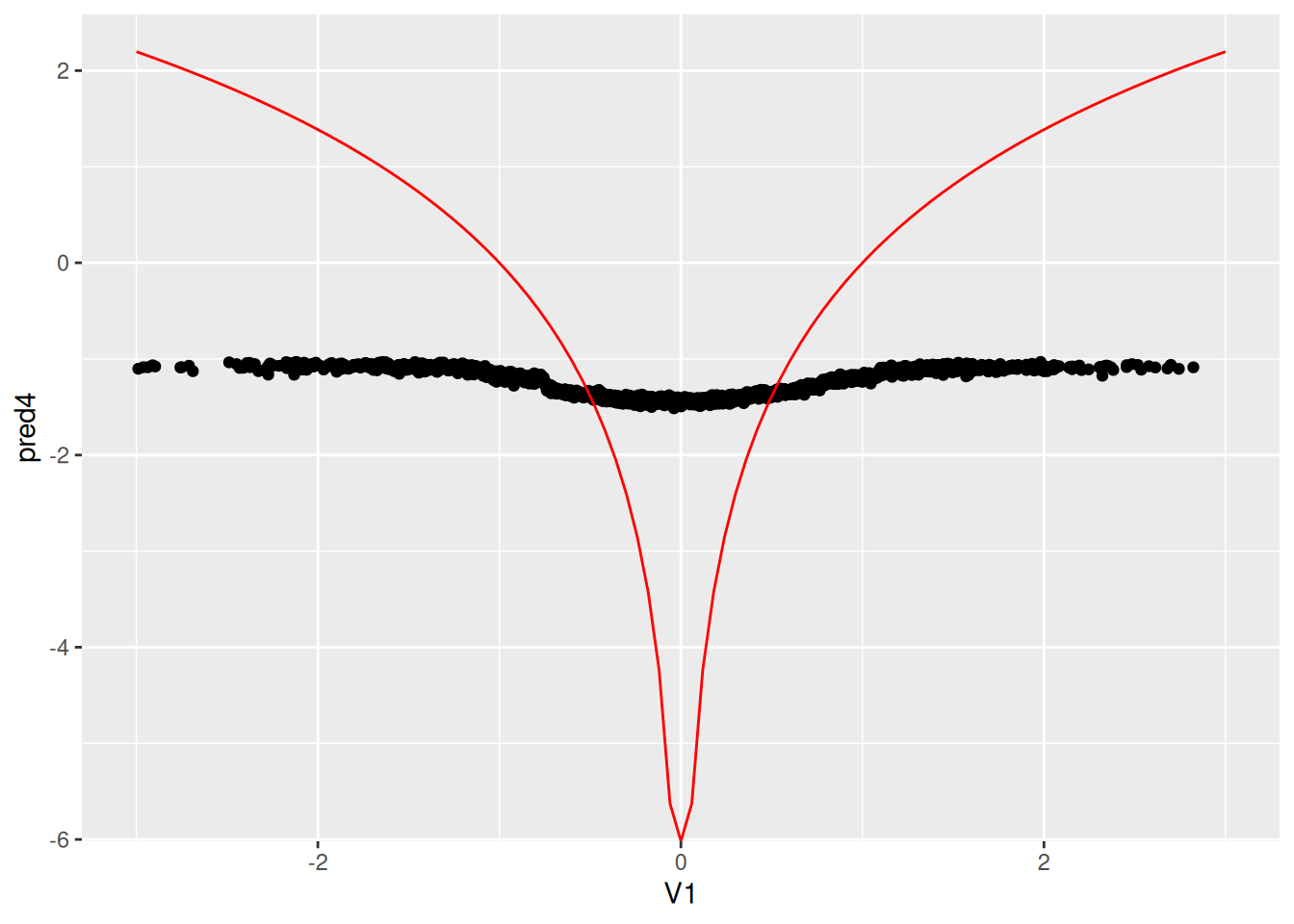
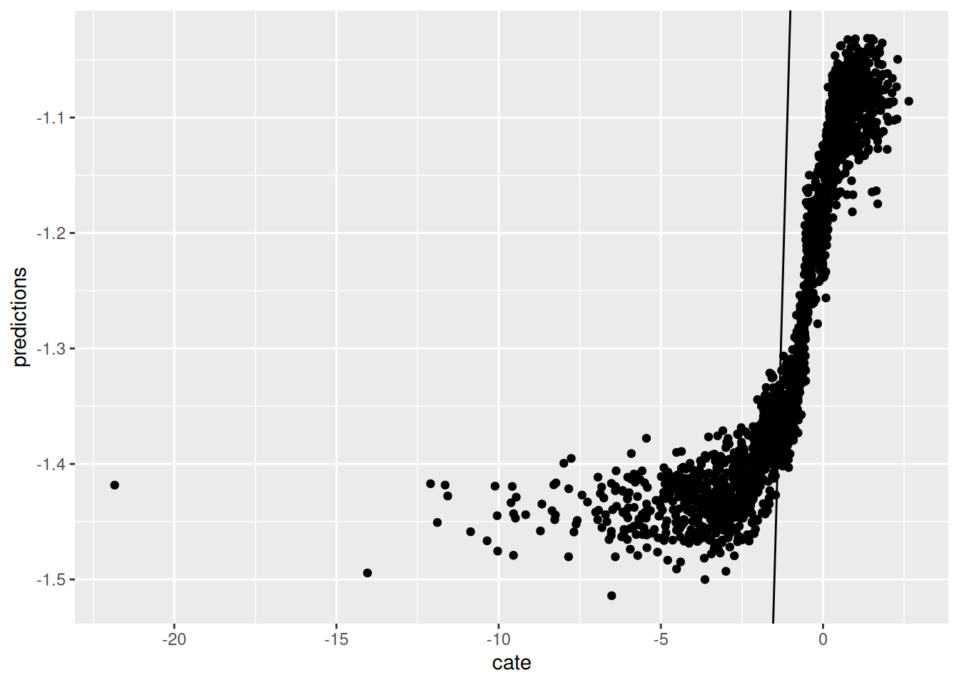
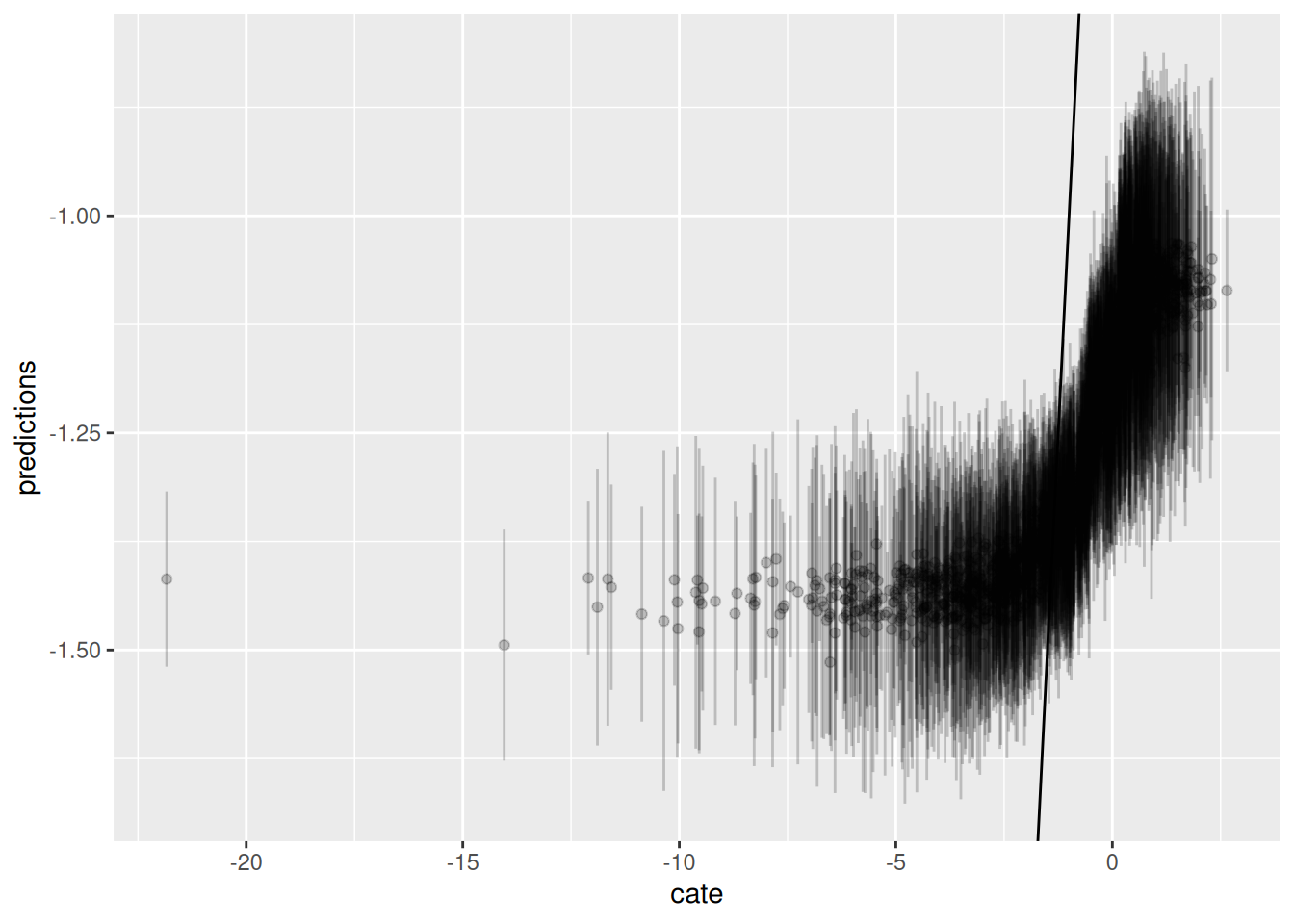
Now we run Causal Forest. Again, first graph is predicted CATE against $V1$, the second one is the predicted CATE against true CATE, the third one adds error bars.
```{r}
#| label: chunk7
#| warning: false
#| cache: true
#| message: false
all_firms <- levels(factor(data$firm))
data.train$firm <- factor(data.train$firm, levels = all_firms)
data.test$firm <- factor(data.test$firm, levels = all_firms)

# a is a data set of firm dummies
a <- as.data.frame(model.matrix(y~firm,data.train))
X <- as.matrix(bind_cols(data.train[,c(5,7:16)],a))
Y <- data.train$y
W <- data.train$W

#tau.forest = causal_forest(X, Y, W, num.trees = 4000)
a <- as.data.frame(model.matrix(y~firm,data.test))
X.test <- as.matrix(bind_cols(data.test[,c(5,7:16)],a))
Y.test <- data.test$y
W.test <- data.test$W

tau.forest4 = causal_forest(X, Y, W, clusters = as.integer(data.train$firm))

average_treatment_effect(tau.forest4, target.sample = "all")
average_treatment_effect(tau.forest4, target.sample = "treated")
#tau.forest3 = causal_forest(X, Y, W, num.trees = 4000)
tau.hat4 = predict(tau.forest4, X.test, estimate.variance = TRUE)
sigma.hat4 = sqrt(tau.hat4$variance.estimates)

data.test$pred4 <- tau.hat4$predictions

fun.1 <- function(x) log(x^2)
ggplot(data.test, aes(x=V1, y=pred4)) + geom_point() +
stat_function(fun = fun.1, colour="red") + xlim(-3,3)
graph.data4 <- as.data.frame(tau.hat4)
graph.data4 <- graph.data4 %>%
    mutate(cate=log(data.test$V1^2)) %>%
    mutate(lower=predictions - sigma.hat4, upper=predictions + sigma.hat4)

ggplot(graph.data4, aes(x=cate, y=predictions)) + geom_point()  + geom_abline(slope = 1)
ggplot() + geom_errorbar(graph.data4, mapping=aes(x=cate, ymin=lower,ymax=upper), alpha = 0.2) + geom_point(graph.data4, mapping=aes(x=cate, y=predictions), alpha = 0.2) + geom_abline(slope = 1)
```
## Summary
We see in these examples, Causal Forest performs fairly well, while other linear models will not work in the nonlinear DGP situations.
---
<!-- see-also-footer -->
*Systematic treatment: [R](https://xiangao.github.io/causal_econometrics_guide/heterogeneous-effects.html) · [Julia](https://xiangao.github.io/causal_econometrics_julia/heterogeneous-effects.html).*