---
title: "G-computation (g-formula) with time varying covariates"
date: "2024-04-20"
---
## The problem
The g-formula (g-computation algorithm) is a method to estimate the causal effect of a time varying treatment or covariates, developed by Robins (1986). Note this is distinct from **g-estimation** of structural nested models (Robins and Rotnitzky, 1992), a different g-methods estimator that uses instrumental-variable-like estimating equations and does not require modeling the joint distribution of all time-varying confounders. This chapter — and the `gfoRmula`/`gmethods` packages used below — implements the g-formula, not g-estimation.
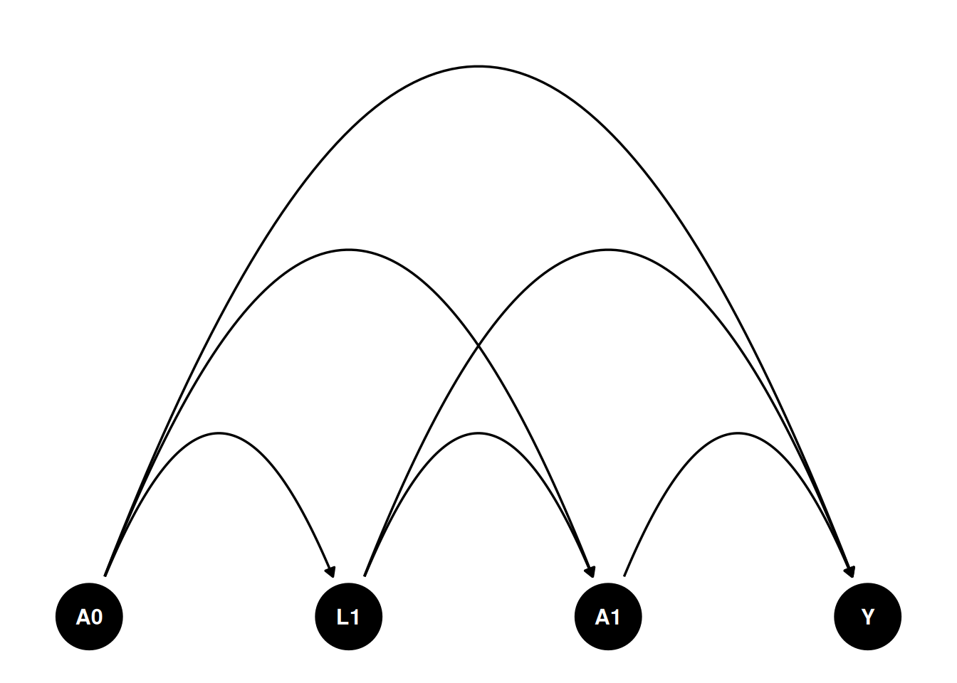
We can imagine such a scenario. Suppose $A0$ and $A1$ are time 0 and time 1 treatment, can be binary or continuous. $L1$ is a time 1 covariate. It can be some intermediate outcome. Say HbA1c. HbA1c can be a result of treatment $A0$. Then it can be a cause for the next period treatment $A1$. $Y$ is the outcome. $U$ is the unmeasured confounder. The causal diagram is shown below. How do we estimate the effect of treatment?
```{r}
#| message: false
#| warning: false
#| cache: true
library(dagitty)
library(ggdag)
library(ggplot2)
library(gfoRmula)
library(gmethods)
library(tidyverse)

dag <- dagify(
  Y ~ A1 + A0 + L1 ,
  A1 ~ A0 + L1,
  L1 ~ A0 ,
  coords = time_ordered_coords()
)

dag %>%
  ggplot(aes(x = x, y = y, xend = xend, yend = yend)) +
  geom_dag_point() +
  geom_dag_edges_arc() +
  geom_dag_text() +
  theme_dag()
```
## Assumptions
There are four potential outcomes, with $A_0$ and $A_1$ can be 0 or 1. The causal estimand is
$$ \tau_{a_0,a_1,a_0',a_1'} = E[Y^{a_0,a_1} - Y^{a_0',a_1'}]$$
To identify the effects, we need assumptions.
1. Sequential ignorability
$$ Y^{a_0,a_1} \perp A_0$$
$$ Y^{a_0,a_1} \perp A_1^{a_0} | A_0, L_1^{a_0}$$
In general, treatment at time $t$ is randomized with probabilities depending on the observed past (covariates and intermediate outcomes): at any time $t$, for every regime $\bar a$,
$$ Y^{\bar a} \perp A_t \mid H_t $$
where $H_t$ is the **observed** history of treatment and covariates up to time $t$,
$$H_t=(A_0, A_1, ..., A_{t-1}; L_1,..., L_{t}).$$
Read this in terms of the *observed* treatment $A_t$ and the *observed* history $H_t$: conditional on what has actually happened up to time $t$, the next treatment is independent of the future potential outcome. The superscripted objects in the two-period statement above (e.g. $A_1^{a_0}$, $L_1^{a_0}$) denote the values that would arise under setting $A_0=a_0$; by consistency these equal the observed $A_1$, $L_1$ on the subset of units with $A_0=a_0$, which is what lets the conditional-independence statement be checked on observed data.
2. Positivity
$$ 0 < P(A_0=1) < 1$$
$$ 0 < P(A_1=1|A_0=1, L_1) < 1$$
In general,
$$ 0 < P(A_t=1|H_t) < 1$$
3. Consistency
$$ Y^{a_0,a_1} = Y | (A_0=a_0,A_1=a_1)$$
## Identifiability
$$ \begin{align}
E[Y^{a_0,a_1}] &= E[Y^{a_0,a_1} | A_0=a_0] \\
&= E[Y^{A_0,a_1} | A_0=a_0] \\
&= \sum_{l=0,1}E[Y^{A_0,a_1} | A_0=a_0, L=l] P(L=l | A_0=a_0) \\
&= \sum_{l=0,1}E[Y^{A_0,a_1} | A_0=a_0, L=l, A_1=a_1] P(L=l | A_0=a_0) \\
&= \sum_{l=0,1}E[Y^{A_0,A_1} | A_0=a_0, L=l, A_1=a_1] P(L=l | A_0=a_0)
\end{align} $$
This can be expanded to the general case. Basically start from the first period, then the second, based on the first, and so on.
## Estimation
There are two types of components in the g-estimation. The first is the outcome model, then there are models for time-varying covariates, or intermediate outcomes (confounders).
## Parametric g-formula
In this simple case, if $Y$ is continuous, we can use a linear model. If $Y$ is binary, we can use a logistic model.
$$ E[Y | A_0, A_1, L_1] = \beta_0 + \beta_1 A_0 + \beta_2 L_1 + \beta_3 A_1$$
Suppose $L_1$ is binary,
$$P(L_1=1 | A_0) = logit^{-1}(\gamma_0 + \gamma_1 A_0)$$
$$ L_1 | A_0 \sim Bernoulli\big(logit^{-1}(\gamma_0 + \gamma_1 A_0)\big)$$
We may need to simulate the distribution of the time-varying covariates for the expected value of the potential outcomes.
## an example
I am following Christopher Boyer's example in his teaching page: https://christopherbboyer.com/about.
The first example is from his lab3 teaching page.
First we set up a simulated data set.
```{r}
#| message: false
#| warning: false
#| cache: true
# setting up the data -----------------------------------------------------

# The code below creates the frequency table, and then turns it into long format
# data. Read through the code carefully and run it.

# re-create the frequency table for homework 3
hw3_freq <- tribble(
  ~A_0, ~L_1, ~A_1, ~N, ~Y_1,
  0, 0, 0, 6000, 60,
  0, 0, 1, 2000, 60,
  0, 1, 0, 2000, 210,
  0, 1, 1, 6000, 210,
  1, 0, 0, 3000, 240,
  1, 0, 1, 1000, 240,
  1, 1, 0, 3000, 120,
  1, 1, 1, 9000, 120
)

# expand the frequency table to 1 row per person
# (first just assign everyone the average Y value)
dat <- uncount(hw3_freq, N) %>%
  # give those rows an id number
  rowid_to_column(var = "id") %>%
  # for each of the variables except for id, split it into two
  # rows, one for each time point
  pivot_longer(-id,
               names_to = c(".value", "time"),
               names_sep = "_"
  ) %>%
  # make sure that time is read as a number
  mutate(time = parse_number(time),
         # add some random error to Y
         # (nrow(.) means a different value for each row of the dataset in use
         Y = Y + rnorm(nrow(.), 0, 10))


# create lagged variables
# group_by(id) makes this robust to row order -- lag() would otherwise
# silently lag across a different person's rows if dat were ever re-sorted
# (e.g. by time first). Currently harmless here since dat is in id-major
# order with exactly one row per id per time, but safer to be explicit.
t1 <- dat %>%
  group_by(id) %>%
  mutate(lag_A = lag(A)) %>%
  ungroup() %>%
  filter(time == 1)
```
Then calculate the g-formula by hand.
First for $E[Y^{1,1}]$.
```{r}
#| message: false
#| warning: false
#| cache: true
# fit models for covariate and outcome given past on t1
L_mod <- glm(L ~ lag_A, data = t1, family = binomial())
Y_mod <- glm(Y ~ A * lag_A * L, data = t1)

# create new data set with space for 10,000 simulated entries
nsim <- 10000
baseline_pop <- tibble(id = 1:nsim)

# fix intervention values in the new data set to be consistent with the regime
new_dat_11 <- baseline_pop %>%
  mutate(lag_A = 1, A = 1)

# predict covariate means at time 1
new_dat_11$pL <- predict(L_mod, newdata = new_dat_11, type = "response")

# simulate covariate values at time 1
new_dat_11$L <- rbinom(nsim, 1, new_dat_11$pL)

# predict outcome at time 1 based on simulated covariates and fixed treatments
new_dat_11$Ey <- predict(Y_mod, newdata = new_dat_11, type = "response")

# take mean across all simulations to get g-formula estimate!
mean(new_dat_11$Ey)
```
Then for $E[Y^{0,0}]$.
```{r}
#| message: false
#| warning: false
#| cache: true
# for 0, 0
new_dat_00 <- baseline_pop %>%
  mutate(lag_A = 0, A = 0)

# predict covariate means at time 1
new_dat_00$pL <- predict(L_mod, newdata = new_dat_00, type = "response")

# simulate covariate values at time 1
new_dat_00$L <- rbinom(nsim, 1, new_dat_00$pL)

# predict outcome at time 1 based on simulated covariates and fixed treatments
new_dat_00$Ey <- predict(Y_mod, newdata = new_dat_00, type = "response")

# take mean across all simulations to get g-formula estimate!
mean(new_dat_00$Ey)
```
Now with the gfoRmula package.
```{r}
#| message: false
#| warning: false
#| cache: true
# running the g-formula ---------------------------------------------------

# add your comments to the lines below
id <- "id"
time_name <- "time"
covnames <- c("L", "A")
outcome_name <- "Y"
#
outcome_type <- "continuous_eof"
#
histories <- c(lagged)
#
histvars <- list(c("A"))
#
covtypes <- c("binary", "binary")
covparams <- list(covmodels = c(
  L ~ lag1_A,
  A ~ lag1_A * L
))
ymodel <- Y ~ A * L * lag1_A
#
intvars <- list("A", "A", "A", "A")
#
interventions <- list(
  list(c(static, c(0, 0))),
  list(c(static, c(0, 1))),
  list(c(static, c(1, 0))),
  list(c(static, c(1, 1)))
)
int_descript <- c(
  "0, 0",
  "0, 1",
  "1, 0",
  "1, 1"
)

# put it all together
# (the warning "obs_data was coerced to a data table" is fine!)
gform_res <- gfoRmula::gformula(
  obs_data = dat,
  id = id,
  time_name = time_name,
  covnames = covnames,
  outcome_name = outcome_name,
  outcome_type = outcome_type,
  covtypes = covtypes,
  covparams = covparams,
  ymodel = ymodel,
  intvars = intvars,
  interventions = interventions,
  int_descript = int_descript,
  ref_int = 1,
  histories = histories,
  histvars = histvars,
  sim_data_b = TRUE,
  seed = 345636
)
# Use the following code to explore the results. (You can ignore Intervention 0,
# the natural course intervention, for now.) How many models were fit? How can
# you tell which of the data in the `sim_data` object was simulated or predicted
# from a model? Does these results match your answers to the earlier questions,
gform_res
gform_res$coeffs
gform_res$sim_data
```
## A second example
Chistopher Boyer has a package "gmethods" that can be used to estimate the g-formula. To me it's a bit more intuitive than the gfoRmula package. Here is an example in the "gmethods" package, with the same model in the "gfoRmula" package.
The example dataset continuous_eofdata again consists of 7,500 observations on 2,500 individuals with a maximum of 7 follow-up times, where the outcome corresponds to a characteristic only in the last interval (e.g., systolic blood pressure in interval 7). The variables in the dataset are:
t0: The time index
id: A unique identifier for each individual
L1: A time-varying covariate; categorical
L2: A time-varying covariate; continuous
L3: A baseline covariate; continuous
A: The treatment variable; binary
Y: The outcome of interest; continuous
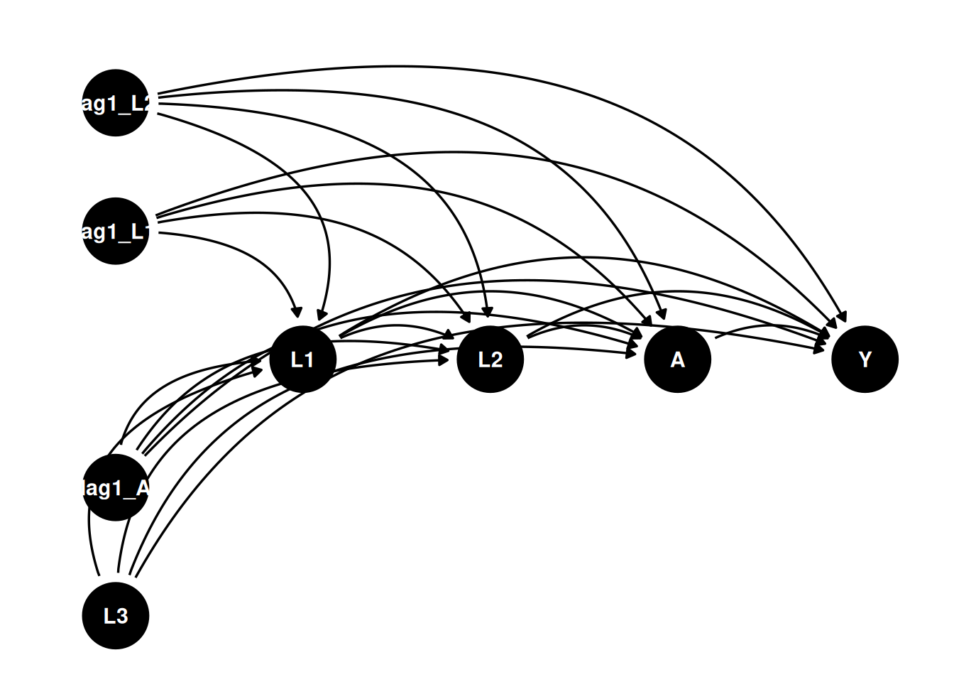
The goal is to estimate the mean outcome at time $K + 1 = 7$ under ‘‘never treat’’ versus ‘‘always treat.’’
The DAG would be something like:
```{r}
#| message: false
#| warning: false
#| cache: true
dag <- dagify(
  Y ~ A + L1 + L2 + L3 + lag1_A + lag1_L1 + lag1_L2 ,
  L1 ~ lag1_A + lag1_L1 + lag1_L2 + L3 ,
  L2 ~ lag1_A + L1 + lag1_L1 + lag1_L2 + L3,
  A ~ lag1_A + L1 + L2 + lag1_L1 + lag1_L2 + L3,
  coords = time_ordered_coords()
)

dag %>%
  ggplot(aes(x = x, y = y, xend = xend, yend = yend)) +
  geom_dag_point() +
  geom_dag_edges_arc() +
  geom_dag_text() +
  theme_dag()
```
### gFormula results
First use the gFormula package.
```{r}
#| message: false
#| warning: false
#| cache: true
id <- 'id'
time_name <- 't0'
covnames <- c('L1', 'L2', 'A')
outcome_name <- 'Y'
covtypes <- c('categorical', 'normal', 'binary')
histories <- c(lagged)
histvars <- list(c('A', 'L1', 'L2'))
covparams <- list(covmodels = c(L1 ~ lag1_A + lag1_L1 + L3 + t0 +
                                 lag1_L2,
                                L2 ~ lag1_A + L1 + lag1_L1 + lag1_L2 + L3 + t0,
                                A ~ lag1_A + L1 + L2 + lag1_L1 + lag1_L2 + L3 + t0))
ymodel <- Y ~ A + L1 + L2 + lag1_A + lag1_L1 + lag1_L2 + L3
intvars <- list('A', 'A')
interventions <- list(list(c(static, rep(0, 7))),
                      list(c(static, rep(1, 7))))
int_descript <- c('Never treat', 'Always treat')
nsimul <- 50000

gform_cont_eof <- gformula_continuous_eof(obs_data = continuous_eofdata,
                                          id = id,
                                          time_name = time_name,
                                          covnames = covnames,
                                          outcome_name = outcome_name,
                                          covtypes = covtypes,
                                          covparams = covparams, ymodel = ymodel,
                                          intvars = intvars,
                                          interventions = interventions,
                                          int_descript = int_descript,
                                          histories = histories,
                                          histvars = histvars,
                                          model_fits = TRUE,
                                          basecovs = c("L3"),
                                          nsimul = nsimul, seed = 1234)
gform_cont_eof
```
### gmethods results
Now use the gmethods package.
```{r}
#| message: false
#| warning: false
#| cache: true
gf <- gmethods::gformula(
  outcome_model = list(
    formula = Y ~ A + L1 + L2 + lag1_A + lag1_L1 + lag1_L2 + L3,
    link = "identity",
    family = "normal"
  ),
  covariate_model = list(
    "L1" = list(
      formula = L1 ~ lag1_A + lag1_L1 + L3 + t0 + lag1_L2,
      family = "categorical"
    ),
    "L2" = list(
      formula = L2 ~ lag1_A + L1 + lag1_L1 + lag1_L2 + L3 + t0,
      link = "identity",
      family = "normal"
    ),
    "A" = list(
      formula = A ~ lag1_A + L1 + L2 + lag1_L1 + lag1_L2 + L3 + t0,
      link = "logit",
      family = "binomial"
    )
  ),
  data = continuous_eofdata,
  survival = FALSE,
  id = 'id',
  time = 't0'
)

s <- simulate(
  gf,
  interventions = list(
    "Never treat" = function(data, time) set(data, j = "A", value = 0),
    "Always treat" = function(data, time) set(data, j = "A", value = 1)
  ),
  n_samples = 50000
)

s$results
```
Note the results are very close. Also note that in the covariates and treatment models, there is a time variable t0. This is because these models are pooled regression with all time points. Therefore a time fixed effect is included. In the outcome model, there is only the last period data, so the time variable is not included.
Standard errors can be calculated with bootstrapping.
---
<!-- see-also-footer -->
*Systematic treatment: [R](https://xiangao.github.io/causal_econometrics_guide/g-methods.html) · [Julia](https://xiangao.github.io/causal_econometrics_julia/g-methods.html).*