34 Simulation on proximal causal inference with panel data
This chapter extends proximal causal inference to a panel-data setting. The question is whether lagged treatment and lagged outcome can serve as negative control exposure (NCE) and negative control outcome (NCO), respectively, to account for unobserved confounders.
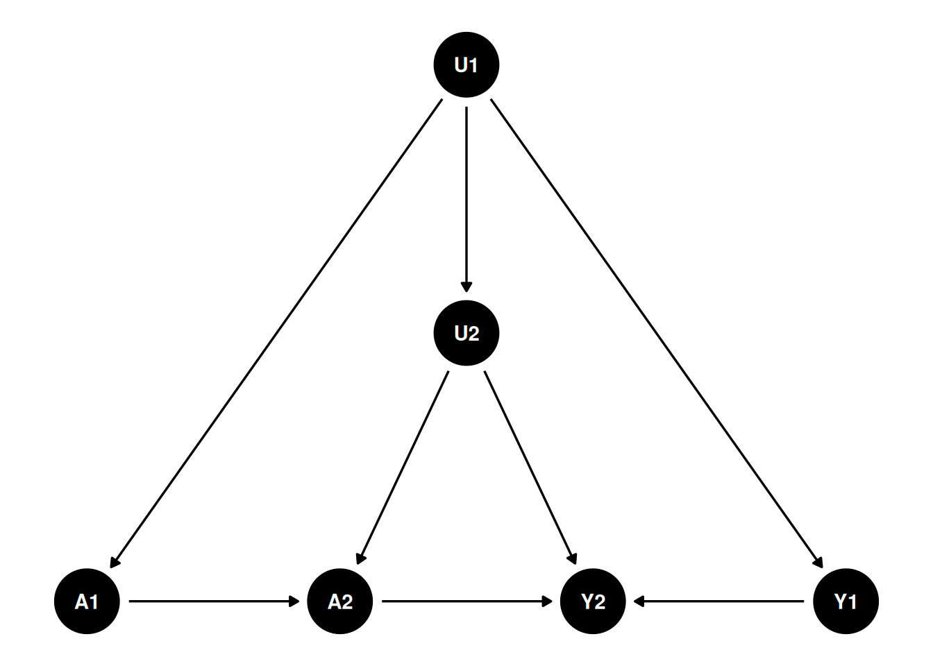
Consider a two-period DAG:
Suppose that’s the case for the causal structure, then I can reasonably combine U1 and U2 into a single unobserved confounder \(U\):
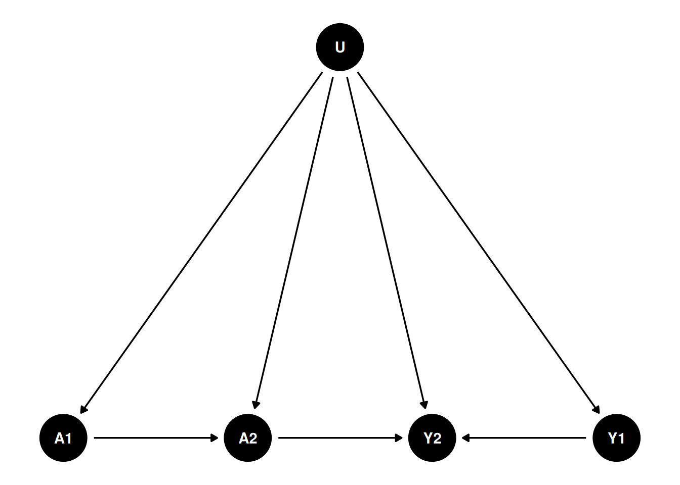
That would fit into the double negative control framework. The problem is that we have to assume there is no link from A1 to Y1, which is odd. Can we assume in period 1 there is no effect, but in period 2, there is an effect?
34.1 A simulation with panel data
I generate two period data based on the DAG above.
Code
library(dplyr)
library(rootSolve)
library(tidyverse)

gen_data <- function(seed, n){
  set.seed(seed)
  u <- rnorm(n, mean = 0, sd = 1)  # unobserved confounder
  x1 <- rnorm(n, mean = 0, sd = 1)  # observed confounder
  x2 <- rnorm(n, mean = 0, sd = 1)  # observed confounder
  a1 <- rbinom(n, 1, plogis(2*u + 1.5*x1))  # treatment at time 1
  a2 <- rbinom(n, 1, plogis(u + a1 +  x1))  # treatment at time 2
  y1 <-  1.5*u + .5*x1  +  rnorm(n, mean = 0, sd = 1)  # outcome at time 1
  y2 <-  y1 + 2.5*u + 2.5*x1 + 3*a2 + rnorm(n, mean = 0, sd = 1)  # outcome at time 2
  data <- data.frame(u=u, x1=x1, x2=x2, a1=a1, a2=a2, y1=y1, y2=y2)
  return(data)
}
data <- gen_data(333, 100000)The simulation draws \(n = 100{,}000\) two-period observations. There is an unobserved confounder \(u \sim N(0,1)\) and two observed covariates \(x_1, x_2 \sim N(0,1)\). Treatment at time 1 is \(a_1 \sim \text{Bernoulli}(\Lambda(2u + 1.5x_1))\) and at time 2 is \(a_2 \sim \text{Bernoulli}(\Lambda(u + a_1 + x_1))\). The outcomes are \(y_1 = 1.5u + 0.5x_1 + \varepsilon_1\) and \(y_2 = y_1 + 2.5u + 2.5x_1 + 3a_2 + \varepsilon_2\).
So the effect of interest is the 3 on \(a_2\). The construction then relabels \(a_1\) as the negative control exposure \(z\) and \(y_1\) as the negative control outcome \(w\) — note that \(y_1\) does not depend on \(a_1\), which is exactly the assumption discussed at the end of this chapter.
We can use the simple 2sls:
Code
Call:
lm(formula = y ~ a + x + what, data = data_sim)

Residuals:
     Min       1Q   Median       3Q      Max
-16.4284  -2.3083   0.0071   2.3020  20.7590

Coefficients:
            Estimate Std. Error t value Pr(>|t|)
(Intercept) -0.01293    0.02315  -0.558    0.577
a            3.02113    0.03528  85.625   <2e-16 ***
x            1.67203    0.01245 134.327   <2e-16 ***
what         2.66578    0.01747 152.631   <2e-16 ***
---
Signif. codes:  0 '***' 0.001 '**' 0.01 '*' 0.05 '.' 0.1 ' ' 1

Residual standard error: 3.456 on 99996 degrees of freedom
Multiple R-squared:  0.6822,    Adjusted R-squared:  0.6822
F-statistic: 7.155e+04 on 3 and 99996 DF,  p-value: < 2.2e-16
The 2SLS coefficient on \(a\) is 3.021 with a standard error of 0.035, against the true 3. The coefficient on the fitted proxy what is 2.666, which is the ratio of the confounder’s loading on the outcome to its loading on the proxy, not an effect of interest.
Or we can use more sophisticated methods. Here I use the m-estimation code by Paul Zivich: https://github.com/pzivich/publications-code/blob/master/ProximalCI/proximal_sims_r.R. This code is to construct estimating equations, then use root finding to find the parameter estimates.
Code
pcl_m2 <- function(theta, mydata, out = "ef"){
  # read in variables
  a <- mydata$a
  x <- mydata$x
  w <- mydata$w
  z <- mydata$z
  y <- mydata$y
  # model for what
  what <- theta[1] + theta[2] * a + theta[3] * x + theta[4] * z

  # matrix of covars in model for what
  wmat <- as.matrix(cbind(rep(1, nrow(mydata)), a, x, z), ncol = 4,
                    nrow = nrow(mydata))

  # estimating function for what
  ef1 <- (t(wmat)  %*% (w - what))            # gives px1 vector (summed over units)
  ef1_b <- wmat * (w - what)                  # gives nxp matrix (rows are units)

  # model for yhat
  yhat <- theta[5] + theta[6]*a + theta[7]*x + theta[8] * what

  # matrix of covars in model for yhat
  ymat <- as.matrix(cbind(rep(1, nrow(mydata)), a, x, what), ncol = 4,
                    nrow = nrow(mydata))

  #estimating function for yhat
  ef2 <- t(ymat) %*% (y - yhat)               # px1 vector, summed over units
  ef2_b <- (ymat) * (y - yhat)                # nxp matrix (rows are units)
  f <- c(ef1, ef2)                            # p-dimensional vector
  if(out == "full") return(cbind(ef1_b, ef2_b)) else return(f) # full used in var calculation only
}

# call m-estimator for PCL
mpcl_mest <- function(dat){
  theta_start <- rep(.05, 8)
  results <- mestimator(pcl_m2, init = theta_start, dat, mydata = dat)
  return(results)
}

##' M-estimation engine
mestimator <- function(ef, init, dat, ...){
  # get estimated coefficients
  fit <- multiroot(ef, start = init, out = "ef",
                   rtol = 1e-9, atol = 1e-12, ctol = 1e-12, ...  )
  betahat <- fit$root
  n <- nrow(dat)

  # bread
  # derivative of estimating function at betahat
  pd <- gradient(ef, betahat, out = "ef", ...)
  pd <- as.matrix(pd)
  bread <- -pd/n
  se_mod <- sqrt(abs(diag(-solve(pd))))

  # meat1
  efhat <- ef(betahat, out = "full", ...)
  meat <- list()
  meat1 <- (t(efhat) %*% efhat)/n

  # sandwich
  sandwich1 <- (solve(bread) %*% meat1 %*% t(solve(bread)))/n
  se_sandwich1 <- sqrt(diag(sandwich1))

  results <- data.frame(betahat, se_sandwich1, se_mod)
  return(results)
}
6 3.021126 0.0198433Code
#mpcl_mest(data_sim)The m-estimator gives 3.0211 with a standard error of 0.0198.
Both the 2sls and the m-estimation give us the same estimate of the causal effect of treatment on outcome, which is 3 — identical to four decimal places, 3.021126 either way. The standard errors differ, 0.0198 against 0.0353, and the m-estimator’s is the one to use: it accounts for the estimation of the first stage, which the plug-in 2SLS standard error does not. The m estimator can be more general. 2sls is good for the linear case.
However, the main issue is the assumption that there is no link from A1 to Y1.
To think about it from a different angle: this is similar to DiD setting. Basically we need A1 to be 0. There is no effect in period 1. If we only have A1 as 0, then it makes sense to have no link from A1 to Y1 (no anticipation assumption).
This is a restrictive identifying assumption, not a technical footnote. Using \(A_{t-1}\) as the negative control exposure and \(Y_{t-1}\) as the negative control outcome only identifies the effect if two separate exclusions hold: \(A_1\) must have no direct effect on \(Y_1\), so that \(Y_1\) is a clean proxy for \(U\) rather than a partly post-treatment quantity; and \(A_1\) must have no direct effect on \(Y_2\) except through \(U\), which is the exclusion restriction that makes \(A_1\) admissible as a negative control exposure in the first place. If either link is actually present — for example, if treatment has an immediate effect in the same period it starts, which is the empirically common case — this proximal construction is misspecified and the estimate above should not be trusted. Before applying this approach, researchers should have a substantive reason to believe treatment effects only appear with a lag.