Code
library(CausalModel)
library(knitr)
set.seed(42)Most causal inference methods assume SUTVA: one unit’s treatment does not affect another unit’s outcome. This is often not true. Vaccinating your neighbor can reduce your risk of infection. A job training program for one worker may affect another worker’s job prospect. A student’s test score may depend on whether classmates received tutoring.
Partial interference (Sobel, M.E. (2006), “What Do Randomized Studies of Housing Mobility Demonstrate?”, Journal of the American Statistical Association, 101(476); Hudgens, M.G. & Halloran, M.E. (2008), “Toward Causal Inference With Interference”, Journal of the American Statistical Association, 103(482)) is one way to make this manageable. Units are organized into clusters. Interference can happen within a cluster, but not between clusters. This is still a strong assumption, but it is weaker than no interference.
Qu et al. (2021) develop clustered IPW and AIPW estimators for this setting – see the CausalModel R package’s documentation/vignette for the exact reference. Here I just simulate data and see how the functions work.
Each unit \(i\) belongs to a cluster \(c\), such as a household, classroom, or village. Within each cluster, units are also organized into groups indexed by \(j = 0, 1, \ldots, J-1\). The group structure \(\mathbf{s} = (s_0, s_1, \ldots, s_{J-1})\) gives the number of units per group.
For example, with group_struct = c(2, 3):
The groups can be real roles, such as parents and children, or they can just be a modeling device.
The key object is the neighborhood configuration \(G_i = (g_0, g_1, \ldots, g_{J-1})\). Here \(g_j\) counts how many other units in group \(j\) within unit \(i\)’s cluster are treated. “Other” means excluding unit \(i\) itself.
With group_struct = c(2, 3):
Under partial interference, the treatment effect for unit \(i\) depends on its neighborhood \(G_i\):
\[\beta(G) = E[Y_i(1, G) - Y_i(0, G)] \tag{43.1}\]
where \(Y_i(z, G)\) is unit \(i\)’s potential outcome when its own treatment is \(z\) and its neighborhood configuration is \(G\).
A simple model is to make the treatment effect linear in the neighborhood:
\[\beta(G) = \tau + \sum_{j=0}^{J-1} \gamma_j \cdot g_j \tag{43.2}\]
where:
With group_struct = c(2, 3), \(\tau = 1\), \(\gamma_0 = 0.5\), \(\gamma_1 = 0.1\):
| Neighborhood \(G\) | Formula | \(\beta(G)\) |
|---|---|---|
| \((0, 0)\) | \(1 + 0 \times 0.5 + 0 \times 0.1\) | 1.0 |
| \((1, 0)\) | \(1 + 1 \times 0.5 + 0 \times 0.1\) | 1.5 |
| \((0, 1)\) | \(1 + 0 \times 0.5 + 1 \times 0.1\) | 1.1 |
| \((1, 1)\) | \(1 + 1 \times 0.5 + 1 \times 0.1\) | 1.6 |
Having one treated neighbor in group 0 adds 0.5 to the treatment effect; having one in group 1 adds only 0.1.
Standard IPW uses one propensity score, \(P(Z_i = 1 | X_i)\). Under interference, we need two:
The second piece is the new part. It models how likely a particular treatment environment is, conditional on covariates.
Note the conditioning on \(Z_i\) in the second piece. Own treatment \(Z_i\) and the neighborhood exposure \(G_i\) are usually dependent by design — for a network or cluster exposure mapping, \(G_i\) is built from the treatments of \(i\)’s neighbours, which are correlated with \(i\)’s own assignment mechanism. The joint exposure probability must therefore be modeled as a joint distribution \(P(Z_i=z, G_i=g \mid X_i)\), or via the valid factorization \(P(Z_i=z\mid X_i)\,P(G_i=g\mid Z_i=z, X_i)\). A product of the two marginals \(P(Z_i\mid X_i)P(G_i\mid X_i)\) is only correct when own and neighborhood treatment are conditionally independent given \(X_i\), which is not the typical case.
The clustered IPW estimator for \(\beta(g)\) reweights outcomes by the joint exposure probability, written here as the conditional factorization:
\[\hat{\beta}_{\text{IPW}}(g) = \frac{1}{N} \sum_i \left[ \frac{\mathbf{1}(Z_i=1, G_i=g)}{P(Z_i=1|X_i) \cdot P(G_i=g|Z_i=1,X_i)} - \frac{\mathbf{1}(Z_i=0, G_i=g)}{P(Z_i=0|X_i) \cdot P(G_i=g|Z_i=0,X_i)} \right] Y_i \tag{43.3}\]
This gives a separate treatment-effect estimate at each neighborhood configuration \(g\).
The AIPW version adds outcome models:
This is the estimator I would usually try first, for the same reason standard AIPW is attractive.
Standard errors are computed by a matching-based variance estimator. Within each group and neighborhood configuration, units are matched on standardized covariates, and the variance is estimated from the matched pairs. This avoids a cluster bootstrap, which can be expensive here.
library(CausalModel)
library(knitr)
set.seed(42)The generate_fixed_cluster() function creates synthetic data where the interference structure is known. We build 200 clusters of 5 units each — 2 in group 0 and 3 in group 1, 1,000 units in all. The direct effect is \(\tau = 1\), and the spillover is 0.5 per treated neighbour in group 0 and 0.1 per treated neighbour in group 1. Treatment prevalence comes out at 0.477.
cdata <- generate_fixed_cluster(
  clusters = 200,
  group_struct = c(2, 3),   # 2 units in group 0, 3 in group 1
  tau = 1,                   # direct effect
  gamma = c(0.5, 0.1)        # spillover: 0.5 per treated in group 0, 0.1 in group 1
)

cat("Total units:", length(cdata$Y), "\n")
Total units: 1000 Units per cluster: 5 Treatment prevalence: 0.477 Each unit has:
Y — observed outcomeZ — treatment indicator (0/1)X — individual covariatescluster_labels — which cluster the unit belongs togroup_labels — which group within the cluster (0-indexed)ingroup_labels — position within the group (0-indexed)cl_obj <- clustered(
Y = cdata$Y,
Z = cdata$Z,
X = cdata$X,
cluster_labels = cdata$cluster_labels,
group_labels = cdata$group_labels,
ingroup_labels = cdata$ingroup_labels,
n_matches = 50
)The clustered() constructor does several things:
result_aipw <- est_via_aipw(cl_obj)The result is a list with one element per group. Each element contains beta_g, the treatment effects at each neighborhood configuration, and se, the standard errors:
for (j in seq_along(result_aipw)) {
cat(sprintf("Group %d:\n", j - 1))
valid <- !is.nan(result_aipw[[j]]$beta_g) & result_aipw[[j]]$se > 0
df <- data.frame(
g_index = which(valid) - 1,
beta_g = round(result_aipw[[j]]$beta_g[valid], 3),
se = round(result_aipw[[j]]$se[valid], 3)
)
print(df, row.names = FALSE)
cat("\n")
}Group 0:
g_index beta_g se
0 0.677 0.364
1 1.572 0.347
3 1.447 0.315
4 1.870 0.257
6 1.141 0.276
7 2.003 0.276
9 1.015 0.428
10 2.674 0.384
Group 1:
g_index beta_g se
0 1.528 0.311
1 1.634 0.228
2 2.126 0.331
3 1.280 0.266
4 1.799 0.188
5 2.180 0.269
6 1.272 0.419
7 2.137 0.247
8 2.850 0.389result_ipw <- est_via_ipw(cl_obj)The neighborhood configurations are encoded as integers. For group_struct = c(2, 3), the encoding for group 0 is:
\[G_{\text{encoded}} = g_0 + g_1 \times (s_0 + 1) \tag{43.4}\]
where \(s_0 = 2\) is the size of group 0. The stride for the second dimension is \(s_0 + 1 = 3\) because the package allocates slots for \(g_0 \in \{0, 1, 2\}\), even though \(g_0 = 2\) is impossible for units in group 0.
| \(g_0\) | \(g_1\) | Encoded | True \(\beta\) |
|---|---|---|---|
| 0 | 0 | 0 | 1.0 |
| 1 | 0 | 1 | 1.5 |
| 0 | 1 | 3 | 1.1 |
| 1 | 1 | 4 | 1.6 |
| 0 | 2 | 6 | 1.2 |
| 1 | 2 | 7 | 1.7 |
Some configurations do not have enough observations. The se > 0 filter removes degenerate cases.
Reading the estimates against that table: configuration 0 (no treated neighbours) gives 0.677 against a true 1.0, configuration 1 gives 1.572 against 1.5, configuration 3 gives 1.447 against 1.1, and configuration 4 gives 1.870 against 1.6. Single-dataset estimates for individual configurations are noisy, which is what the Monte Carlo below is for.
Clustered IPW gives 0.491, 1.591, 1.404, 1.865 and so on across the same configurations — close to the AIPW numbers but not identical, as expected from two different estimators of the same quantities.
Now run a small Monte Carlo. Generate data 100 times, estimate \(\beta(G)\) each time, and check bias, SE calibration, and coverage.
n_clusters <- 200
group_struct <- c(2, 3)
tau_int <- 1
gamma_int <- c(0.5, 0.1)
n_reps <- 100
# True beta(g) function
true_beta <- function(g) tau_int + sum(g * gamma_int)
# Track results for group 0 at three neighborhood configurations
g_indices <- list(c(0, 0), c(1, 0), c(0, 1))
g_encoded <- sapply(g_indices, function(g) {
g[1] + g[2] * (group_struct[1] + 1) + 1 # 1-indexed; stride = max_g0 + 1
})
true_values <- sapply(g_indices, true_beta)
int_results <- array(NA, dim = c(n_reps, length(g_indices), 2),
dimnames = list(NULL, NULL, c("beta", "se")))set.seed(2024)
for (i in seq_len(n_reps)) {
cdata <- generate_fixed_cluster(
clusters = n_clusters, group_struct = group_struct,
tau = tau_int, gamma = gamma_int
)
cl_obj <- clustered(
  Y = cdata$Y,
  Z = cdata$Z,
  X = cdata$X,
  cluster_labels = cdata$cluster_labels,
  group_labels = cdata$group_labels,
  ingroup_labels = cdata$ingroup_labels,
  n_matches = 50
)
res <- est_via_aipw(cl_obj)
for (j in seq_along(g_indices)) {
idx <- g_encoded[j]
int_results[i, j, "beta"] <- res[[1]]$beta_g[idx]
int_results[i, j, "se"] <- res[[1]]$se[idx]
}
}int_rows <- list()
for (j in seq_along(g_indices)) {
betas <- int_results[, j, "beta"]
ses <- int_results[, j, "se"]
valid <- !is.nan(betas) & !is.nan(ses) & ses > 0
betas <- betas[valid]
ses <- ses[valid]
tv <- true_values[j]
ci_lo <- betas - 1.96 * ses
ci_hi <- betas + 1.96 * ses
int_rows[[j]] <- data.frame(
g = paste0("(", paste(g_indices[[j]], collapse = ","), ")"),
True_beta = tv,
Mean_est = mean(betas),
Bias = mean(betas) - tv,
Emp_SE = sd(betas),
Mean_SE = mean(ses),
Coverage = mean(ci_lo <= tv & tv <= ci_hi),
N_valid = length(betas)
)
}
tbl_int <- do.call(rbind, int_rows)
kable(tbl_int, digits = 3, row.names = FALSE,
caption = sprintf("Clustered AIPW (group 0, %d clusters, %d reps)",
n_clusters, n_reps))| g | True_beta | Mean_est | Bias | Emp_SE | Mean_SE | Coverage | N_valid |
|---|---|---|---|---|---|---|---|
| (0,0) | 1.0 | 2.107 | 1.107 | 8.760 | 0.448 | 0.820 | 100 |
| (1,0) | 1.5 | 1.569 | 0.069 | 0.549 | 0.415 | 0.899 | 99 |
| (0,1) | 1.1 | 1.083 | -0.017 | 0.248 | 0.246 | 0.930 | 100 |
Over 100 replications the picture is mixed, and the failure is informative. Configuration \((1,0)\) recovers its truth well — mean 1.569 against 1.5, bias 0.069, coverage 89.9% — and \((0,1)\) better still, 1.083 against 1.1 with 93.0% coverage. But \((0,0)\) is badly behaved: mean 2.107 against a true 1.0, and an empirical standard deviation of 8.760 against a mean reported standard error of 0.448. The estimator is not merely biased there; its own standard error understates the sampling variability by a factor of nearly twenty, and coverage is 82% only because a few enormous outliers drag the mean while most draws sit near the truth.
The reason is positivity. Configuration \((0,0)\) requires a unit with no treated neighbours in either group, and with treatment prevalence near 0.5 in clusters of five that configuration is rare, so the inverse-probability weights attached to it are extreme.
par(mfrow = c(1, length(g_indices)), mar = c(3, 3, 2, 1))
for (j in seq_along(g_indices)) {
  betas <- int_results[, j, "beta"]
  ses <- int_results[, j, "se"]
  valid <- !is.nan(betas) & !is.nan(ses) & ses > 0
  t_stats <- (betas[valid] - true_values[j]) / ses[valid]
  g_label <- paste0("(", paste(g_indices[[j]], collapse = ","), ")")
  hist(t_stats, breaks = 20, freq = FALSE, col = "lightblue",
       main = sprintf("g = %s", g_label),
       xlab = "", xlim = c(-4, 4))
  curve(dnorm(x), add = TRUE, col = "red", lwd = 2)
  abline(v = 0, lty = 2)
}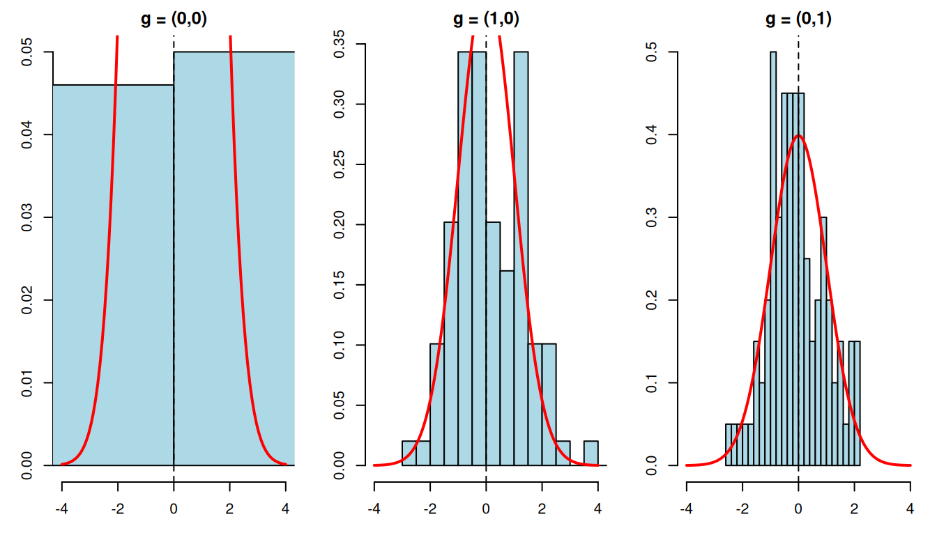
If both the estimator and SE work well, the studentized statistics should look roughly normal.
What happens if we ignore interference and use a standard AIPW estimator? We get one number that averages over neighborhood configurations. That number is hard to interpret.
# Generate one dataset with interference
set.seed(42)
cdata <- generate_fixed_cluster(
  clusters = 200,
  group_struct = c(2, 3),
  tau = 1,
  gamma = c(0.5, 0.1)
)

# Naive: ignore clusters, treat as standard observational data
obs_naive <- observational(cdata$Y, cdata$Z, cdata$X)
naive_ate <- est_via_aipw(obs_naive)

cat("Naive AIPW (ignoring interference):", round(naive_ate$ate, 3), "\n")
Naive AIPW (ignoring interference): 1.611 SE: 0.068 # Correct: use clustered estimator
cl_obj <- clustered(
Y = cdata$Y, Z = cdata$Z, X = cdata$X,
cluster_labels = cdata$cluster_labels,
group_labels = cdata$group_labels,
ingroup_labels = cdata$ingroup_labels,
n_matches = 50
)
result <- est_via_aipw(cl_obj)
cat("Clustered AIPW beta_g (group 0):\n")Clustered AIPW beta_g (group 0): g_index beta_g se
0 0.677 0.364
1 1.572 0.347
3 1.447 0.315
4 1.870 0.257
6 1.141 0.276
7 2.003 0.276
9 1.015 0.428
10 2.674 0.384The naive estimate gives some weighted average of the \(\beta(g)\) values, but it does not tell us how much is direct effect and how much is spillover. The clustered estimator separates those pieces. If spillovers are large, treating clusters may be more effective than treating isolated individuals.
Partial interference is a compromise. We do not assume away spillovers, but we do assume they stay inside clusters. Once we make that assumption, the neighborhood configuration \(G\) becomes part of the estimand. The effect is no longer just treatment versus control; it is treatment versus control under a particular neighborhood treatment environment.
The CausalModel package estimates these effects with clustered IPW and AIPW. The important practical lesson is that a standard AIPW estimate is not a good substitute. It collapses direct effects and spillovers into one number.