This post is to illustrate how to use R to do basic conjoint analysis.
38.1 Conjoint Analysis
Marketing people used to use Sawtooth to do conjoint analysis.
What is conjoint analysis? Here is the intro from Sawtooth:
“Conjoint analysis methods use statistical analysis to compute mathematical representations of survey respondents’ preferences for product features, simulate how attribute changes affect demand, and even predict market acceptance of new products before they launch.
This powerful research methodology has become very popular with market researchers and economists for the valuable insight that few other research methods can provide.”
“Consider the task of purchasing a new vehicle.
When searching for the “right” vehicle, you typically consider a multitude of variables: type, make (brand), model, year, mileage, price, color, accessories packages, etc. You can see how this is a complex choice to make.
How does anyone possibly make such a complicated decision?
You think about what features matter most to you and then make tradeoffs.
For example, one vehicle could be an acceptable make and model, but at a high price point, whereas a second option is not the ideal make and model but has a more palatable price.
The tradeoff in this simple example is whether the make and model is more preferable to a reasonable price, or vice versa.
A conjoint survey captures the relationship between different attributes of a product and how preferable they are both comparatively and when combined.
Because of this, conjoint analysis is the gold standard solution for testing multiple features simultaneously, when limited A/B testing doesn’t go far enough.”
“In simple terms, the conjoint survey design algorithm generates a balanced survey design with product profiles, also known as concepts, formulated to have ideal statistical properties (such as level balance and independence of attributes).
Each profile is made up of multiple conjoined product features (hence, conjoint analysis), such as brand, type, engine, and color, each with systematically varied levels.
These product concepts are then included in a series of questions, usually 8-20, called choice tasks, that make up the conjoint analysis portion of the survey.”
38.2 Example
I am following the example here: https://bookdown.org/lien_lamey/R_tutorial/8-1-data-5.html
library(tidyverse)library(openxlsx)url<-"https://feb.kuleuven.be/lien.lamey/public/rmodule/icecream.xlsx"icecream<-read.xlsx(url)icecream<-icecream%>%pivot_longer(cols =starts_with("Individual"), names_to ="respondent", values_to ="rating")%>%# respondent keeps track of the respondent, rating will store the respondent's ratings, and we want to stack every variable that starts with Individualrename("profile"="Observations")%>%# rename Observations to profilemutate(profile =factor(profile), respondent =factor(respondent), # factorize identifiers Flavor =factor(Flavor), Packaging =factor(Packaging), Light =factor(Light), Organic =factor(Organic))# factorize the ice cream attributesicecream
# A tibble: 150 × 7
   profile   Flavor    Packaging       Light      Organic     respondent  rating
   <fct>     <fct>     <fct>           <fct>      <fct>       <fct>        <dbl>
 1 Profile 1 Raspberry Homemade waffle No low fat Not organic Individual…      1
 2 Profile 1 Raspberry Homemade waffle No low fat Not organic Individual…      6
 3 Profile 1 Raspberry Homemade waffle No low fat Not organic Individual…      5
 4 Profile 1 Raspberry Homemade waffle No low fat Not organic Individual…      1
 5 Profile 1 Raspberry Homemade waffle No low fat Not organic Individual…      2
 6 Profile 1 Raspberry Homemade waffle No low fat Not organic Individual…      7
 7 Profile 1 Raspberry Homemade waffle No low fat Not organic Individual…      7
 8 Profile 1 Raspberry Homemade waffle No low fat Not organic Individual…      5
 9 Profile 1 Raspberry Homemade waffle No low fat Not organic Individual…      1
10 Profile 1 Raspberry Homemade waffle No low fat Not organic Individual…     10
# ℹ 140 more rows
In this example, we have 4 attributes: Flavor, Packaging, Light, and Organic. There are 5, 3, 2, 2 levels correspondingly. Usually we are interested in how much does each level of attributes predict the outcome, say the rating of the icecream. To do this, we would think we’ll need all 532*2=60 combinations of attribute levels to estimate the effect. In that case, we would need data for each combination. This is called full factorial design. The problem of full factorial design is that it might be too costly or not possible if the combination is huge. Instead, conjoint analysis allows us to estimate the effect of each level of each attribute by using a fraction of the combinations. This is done by creating a set of profiles, each of which contains a subset of the levels of the attributes. The profiles are then presented to the respondents, who rate the profiles. The ratings are then used to estimate the effect of each level of each attribute. This is done by regressing the ratings on the levels of the attributes. The coefficients of the regression are the estimates of the effects of the levels of the attributes.
The disadvantage of a fractional factorial design is that some effects are confounded; that is, the effect of one level of an attribute is confounded with the effect of another level of another attribute.
# attribute1, attribute2, etc. are vectors with one element in which we first provide the name of the attribute followed by a semi-colon and then provide all the levels of the attributes separated by semi-colonsattribute1<-"Flavor; Raspberry; Chocolate; Strawberry; Mango; Vanilla"attribute2<-"Package; Homemade waffle; Cone; Pint"attribute3<-"Light; Low fat; No low fat"attribute4<-"Organic; Organic; Not organic"# now combine these different attributes into one vector with c()attributes<-c(attribute1, attribute2, attribute3, attribute4)attributes
The first step in conjoint analysis is to create a design of experiment. This is to use a fraction of all possible combinations of attribute levels to estimate the effect of each level of each attribute. For example, instead of using all 60 icecream profiles, we use 10 profiles.
We use “radiant” package’s “doe” function to create the design of experiment. The “doe” function takes the attributes as input and returns a data frame with the profiles. The “seed” argument is used to fix the random number generator. This is useful if you want to reproduce the same results.
This is a list of efficiency of different number of “trials”. Trials mean combinations of attribute levels. For example, with 10 trials, the efficiency is .389 and it’s unbalanced.
We can see that the only two designs with balanced design are 30 and 60. That’s because 30 and 60 are the only two numbers that can be divided by 5, 3 and 2, all unique number of 5, 3, 3, 2. If the factors are, say, 3, 2, 3. Then the integers that can be divided by 3 and 2 are 6, 12, and 18.
Efficiency is a measure of the information content a design can capture. Efficiency are typically stated in relative terms, as in “design A is 80% as efficient as design B.” In practical terms this means you will need 25% more (the reciprocal of 80%) design A observations (respondents, choice sets per respondent or a combination of both) to get the same standard errors and significance as with the more efficient design B. We used a measure of efficiency called D-Efficiency (Kuhfeld et al. 1994). In this case, the only orthogonal design is the full factorial design of 60 trials.
For example, a trial of 30 has a efficiency of .984, that means it’s 98.4% as efficient as the full factorial design of 60 trials.
From the covariance matrix, we can se that in this 30 profile design, there is a correlation of -.105 between “Light” and “Organic”. That means these two effects are confounded; the design is not orthogonal. That’s why the efficiency is not 1. The D-efficiency is calculated as a function of the determinant of the correlation matrix. The D-efficiency of the full factorial design is 1. The D-efficiency of the 30 profile design is .984. That means the 30 profile design is 98.4% as efficient as the full factorial design.
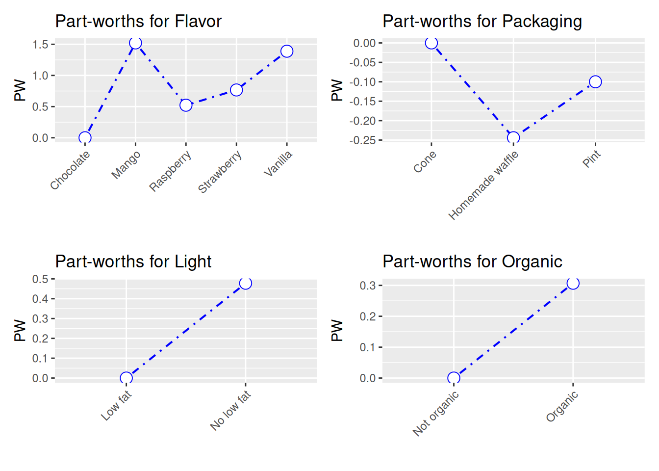
The conjoint importance weights are the relative importance of each attribute. First the range of partworths for each attribute is calculated. Then the range of partworths for each attribute is divided by the sum of the ranges of all attributes. In this example, Flavor is the most important attribute, with an importance weight of .597.
There is another package called “conjoint” which I have not played with.
In summary, we can use R packages to set up a conjoint experiment, in the sense that we can have partial (fractional) factorial design. After collecting the data, we can use either the conjoint packages, or just run linear or logit models to analyze it. The frequentist approach used in conjoint analysis seems nothing special. Bayesian approach can also be used, but that’s another topic.
38.5 Causal effect in conjoint analysis
Hainmueller, Hopkins, and Yamamoto (2014) defined ACME (average marginal component effect). The basic idea is that once all the assumptions are met (usual assumptions in causal inference), we can have the effect of changing one attribute level to another with a causal interpretation. Fortunately it is usually just coefficients from a linear model, or linear combinations of the coefficients. There is a package “cregg” for each calculation and plotting of ACME, but we can just do it manually.
Source Code
---title: "Conjoint design and analysis using R"date: "2024-08-08"execute: freeze: true # radiant is not installable on current R; always use the frozen output---This post is to illustrate how to use R to do basic conjoint analysis. ## Conjoint AnalysisMarketing people used to use Sawtooth to do conjoint analysis.What is conjoint analysis? Here is the intro from Sawtooth:"Conjoint analysis methods use statistical analysis to compute mathematical representations of survey respondents’ preferences for product features, simulate how attribute changes affect demand, and even predict market acceptance of new products before they launch.This powerful research methodology has become very popular with market researchers and economists for the valuable insight that few other research methods can provide.""Consider the task of purchasing a new vehicle.When searching for the “right” vehicle, you typically consider a multitude of variables: type, make (brand), model, year, mileage, price, color, accessories packages, etc. You can see how this is a complex choice to make.How does anyone possibly make such a complicated decision?You think about what features matter most to you and then make tradeoffs.For example, one vehicle could be an acceptable make and model, but at a high price point, whereas a second option is not the ideal make and model but has a more palatable price.The tradeoff in this simple example is whether the make and model is more preferable to a reasonable price, or vice versa.A conjoint survey captures the relationship between different attributes of a product and how preferable they are both comparatively and when combined.Because of this, conjoint analysis is the gold standard solution for testing multiple features simultaneously, when limited A/B testing doesn’t go far enough.""In simple terms, the conjoint survey design algorithm generates a balanced survey design with product profiles, also known as concepts, formulated to have ideal statistical properties (such as level balance and independence of attributes).Each profile is made up of multiple conjoined product features (hence, conjoint analysis), such as brand, type, engine, and color, each with systematically varied levels.These product concepts are then included in a series of questions, usually 8-20, called choice tasks, that make up the conjoint analysis portion of the survey."## ExampleI am following the example here: https://bookdown.org/lien_lamey/R_tutorial/8-1-data-5.html```{r}#| message: false#| warning: false#| cache: truelibrary(tidyverse)library(openxlsx)url <-"https://feb.kuleuven.be/lien.lamey/public/rmodule/icecream.xlsx"icecream <-read.xlsx(url)icecream <- icecream %>%pivot_longer(cols =starts_with("Individual"), names_to ="respondent", values_to ="rating") %>%# respondent keeps track of the respondent, rating will store the respondent's ratings, and we want to stack every variable that starts with Individualrename("profile"="Observations") %>%# rename Observations to profilemutate(profile =factor(profile), respondent =factor(respondent), # factorize identifiersFlavor =factor(Flavor), Packaging =factor(Packaging), Light =factor(Light), Organic =factor(Organic)) # factorize the ice cream attributesicecream```In this example, we have 4 attributes: Flavor, Packaging, Light, and Organic. There are 5, 3, 2, 2 levels correspondingly. Usually we are interested in how much does each level of attributes predict the outcome, say the rating of the icecream. To do this, we would think we'll need all 5*3*2*2=60 combinations of attribute levels to estimate the effect. In that case, we would need data for each combination. This is called full factorial design. The problem of full factorial design is that it might be too costly or not possible if the combination is huge. Instead, conjoint analysis allows us to estimate the effect of each level of each attribute by using a fraction of the combinations. This is done by creating a set of profiles, each of which contains a subset of the levels of the attributes. The profiles are then presented to the respondents, who rate the profiles. The ratings are then used to estimate the effect of each level of each attribute. This is done by regressing the ratings on the levels of the attributes. The coefficients of the regression are the estimates of the effects of the levels of the attributes. The disadvantage of a fractional factorial design is that some effects are confounded; that is, the effect of one level of an attribute is confounded with the effect of another level of another attribute. ```{r}# attribute1, attribute2, etc. are vectors with one element in which we first provide the name of the attribute followed by a semi-colon and then provide all the levels of the attributes separated by semi-colonsattribute1 <-"Flavor; Raspberry; Chocolate; Strawberry; Mango; Vanilla"attribute2 <-"Packaging; Homemade waffle; Cone; Pint"attribute3 <-"Light; Low fat; No low fat"attribute4 <-"Organic; Organic; Not organic"# now combine these different attributes into one vector with c()attributes <-c(attribute1, attribute2, attribute3, attribute4)attributes```## Conjoint design of experimentThe first step in conjoint analysis is to create a design of experiment. This is to use a fraction of all possible combinations of attribute levels to estimate the effect of each level of each attribute. For example, instead of using all 60 icecream profiles, we use 10 profiles. We use "radiant" package's "doe" function to create the design of experiment. The "doe" function takes the attributes as input and returns a data frame with the profiles. The "seed" argument is used to fix the random number generator. This is useful if you want to reproduce the same results.::: {.callout-warning}**Dependency note.** This chapter depends on the `radiant` package, whose plotting functions can fail to install or run on current R versions. If `radiant` is unavailable in your environment, the design-of-experiment and plotting chunks below will not execute; the `doe` output and figures are kept from a prior successful render.:::```{r}#| message: false#| warning: false#| cache: truelibrary(radiant)ice_doe <-doe(attributes, seed =123)ice_doe$eff#summary(doe(attributes, seed = 123, trials = 10))```This is a list of efficiency of different number of "trials". Trials mean combinations of attribute levels. For example, with 10 trials, the efficiency is .389 and it's unbalanced. We can see that the only two designs with balanced design are 30 and 60. That's because 30 and 60 are the only two numbers that can be divided by 5, 3 and 2, all unique number of 5, 3, 3, 2. If the factors are, say, 3, 2, 3. Then the integers that can be divided by 3 and 2 are 6, 12, and 18. Efficiency is a measure of the information content a design can capture. Efficiency aretypically stated in relative terms, as in “design A is 80% as efficient as design B.” Inpractical terms this means you will need 25% more (the reciprocal of 80%) design Aobservations (respondents, choice sets per respondent or a combination of both) to get thesame standard errors and significance as with the more efficient design B. We used ameasure of efficiency called D-Efficiency (Kuhfeld et al. 1994). In this case, the only orthogonal design is the full factorial design of 60 trials. For example, a trial of 30 has a efficiency of .984, that means it's 98.4% as efficient as the full factorial design of 60 trials. ```{r}#| message: false#| warning: false#| cache: truelibrary(radiant)ice_doe2 <-doe(attributes, seed =123, trials =30)ice_doe2$cor_mat```From the covariance matrix, we can se that in this 30 profile design, there is a correlation of -.105 between "Light" and "Organic". That means these two effects are confounded; the design is not orthogonal. That's why the efficiency is not 1. The D-efficiency is calculated as a function of the determinant of the correlation matrix. The D-efficiency of the full factorial design is 1. The D-efficiency of the 30 profile design is .984. That means the 30 profile design is 98.4% as efficient as the full factorial design.The partial factorial design of 30 profile is ```{r}ice_doe2$part```## Conjoint analysisIn the icecream data set we read in, it's a 10 profile design. There are 15 respondents. They rate 10 profiles of icecreams.```{r}#| message: false#| warning: false#| cache: trueconjoint <-conjoint(icecream, rvar ="rating", evar =c("Flavor","Packaging","Light","Organic")) summary(conjoint)``````{r}plot(conjoint)```The partworths are just coefficient from a linear regression:```{r}#| message: false#| warning: falselibrary(sandwich)library(lmtest)partworths_lm <-lm(rating ~ Flavor + Packaging + Light + Organic, data = icecream)summary(partworths_lm)# Each of the 15 respondents rates 10 profiles, so observations are clustered# by respondent; plain OLS standard errors above assume independence and# understate the true uncertainty. Cluster at the respondent level instead.coeftest(partworths_lm, vcov =vcovCL(partworths_lm, cluster = icecream$respondent))```The conjoint importance weights are the relative importance of each attribute. First the range of partworths for each attribute is calculated. Then the range of partworths for each attribute is divided by the sum of the ranges of all attributes. In this example, Flavor is the most important attribute, with an importance weight of .597. There is another package called "conjoint" which I have not played with. In summary, we can use R packages to set up a conjoint experiment, in the sense that we can have partial (fractional) factorial design. After collecting the data, we can use either the conjoint packages, or just run linear or logit models to analyze it. The frequentist approach used in conjoint analysis seems nothing special. Bayesian approach can also be used, but that's another topic. ## Causal effect in conjoint analysisHainmueller, Hopkins, and Yamamoto (2014) defined AMCE (average marginal component effect) -- not to be confused with ACME (average causal mediation effect, Imai et al.), a different causal estimand from the mediation-analysis literature. The basic idea is that once all the assumptions are met (usual assumptions in causal inference), we can have the effect of changing one attribute level to another with a causal interpretation. Fortunately it is usually just coefficients from a linear model, or linear combinations of the coefficients. There is a package "cregg" for each calculation and plotting of AMCE, but we can just do it manually.