library(engression)

# Nonlinear DGP with heteroskedastic noise
n <- 1000
X <- matrix(rnorm(n * 2), ncol = 2)
Y <- (X[,1])^2 + X[,2] + rnorm(n) * (0.5 + abs(X[,1]))

# Fit engression; it learns the full conditional distribution
engr <- engression(X, Y)

# Predict conditional mean (like lm, but nonlinear)
Yhat_mean <- predict(engr, X, type = "mean")

# Predict conditional quantiles (like quantile regression, but joint)
Yhat_quant <- predict(engr, X, type = "quantiles")

# Sample from the learned distribution (generative)
Ysample <- predict(engr, X, type = "sample", nsample = 1)42 Frengression and Engression
In the causal simulation chapter, I used Evans and Didelez (2024)’s decomposition of the joint distribution \(p(x,a,y)\) into three pieces:
\[ p(x,a,y) = p(x,a) \cdot p_a(y) \cdot c(x,y|a) \]
where \(p(x,a)\) is the “past” distribution of covariates and treatment, \(p_a(y)\) is the causal margin, and \(c(x,y|a)\) is the copula linking covariates and outcome given treatment. The causl package implements this with parametric families. We specify Gaussian, binomial, and so on for each piece.
But real data can be hard to specify parametrically. We may not know the right copula family. The marginal distributions may have mass points, skewness, or other features that are annoying to write down.
Frengression (Yang, Evans and Shen, 2025) keeps the same decomposition but learns the pieces with neural networks.
There are two uses: causal simulation with a learned generative model, and interventional prediction using learned confounding structure. The second part uses engression, so I start there.
42.1 Engression
Engression (Shen and Meinshausen, 2024) stands for energy regression. Standard regression estimates \(E[Y|X]\). Engression tries to learn the whole conditional distribution \(P(Y|X)\) using neural networks trained with the energy score.
42.1.1 The Energy Score
The energy score is a proper scoring rule for distributions. Given observations \(Y\) and samples \(\hat Y, \hat Y'\) from the model:
\[ S(Y, \hat Y, \hat Y') = E\|Y - \hat Y\| - \frac{1}{2}E\|\hat Y - \hat Y'\| \]
The first term rewards samples close to the truth. The second term keeps the simulated distribution from collapsing to one point. This is why the method targets the full distribution rather than only the mean.
42.1.2 The Stochastic Network (StoNet)
The building block is a StoNet, a neural network that adds random noise \(\epsilon \sim N(0,I)\) to the input at each layer:
\[\text{StoNet}(x) = f(x, \epsilon), \quad \epsilon \sim N(0,I)\]
Different noise draws produce different outputs. Each output is a sample from the learned conditional distribution. So we can:
- Predict the mean: average over many noise draws → \(E[Y|X=x]\)
- Predict quantiles: take quantiles of the noise draws → conditional quantile regression
- Sample: each forward pass with fresh noise is a sample from \(P(Y|X=x)\)
42.1.3 Why Engression?
Compared with quantile regression or mixture density networks, engression is useful because:
- it handles multivariate responses directly;
- it does not require us to specify a Gaussian mixture or a list of quantiles;
- it gives samples from the conditional distribution, which is convenient for simulation.
42.1.4 Quick Example
The engression R package, separate from Rfrengression, provides the standalone estimator. The code below shows the API. The Rfrengression examples later are the ones I actually run here.
The point is that engression gives a distributional model of \(Y|X\), not just a fitted mean.
42.2 From Engression to Frengression
Frengression is frugal simulation plus engression. It uses three engression models to represent the decomposition of \(P(X,A,Y)\). Each sub-network is trained with the energy score.
42.3 The Architecture
Frengression has three sub-networks, matching the three pieces of the decomposition:
| Decomposition | causl (parametric) | Frengression (neural net) |
|---|---|---|
| \(P(X,A)\) — the past | Specified by family + params |
model_xz: noise-only generator |
| \(P_a(Y)\) — causal margin | Specified by family + params |
model_y: takes \((x, \text{eta})\), outputs \(y\)
|
| \(c(X,Y \mid A)\) — copula | Gaussian/Frank/etc. copula |
model_eta: takes \((x,z)\), outputs eta |
The important part is model_eta. It takes \((x,z)\) and outputs a latent variable eta that carries the dependence between confounders and outcome. During training, a Z-permutation trick forces eta to be marginally \(N(0,I)\). This means:
- When
etacomes frommodel_eta(x,z), it carries the observational confounding information. - When
etais sampled independently from \(N(0,1)\), it gives the interventional prediction.
Same network, different source of eta. That is the trick.
42.4 Using Rfrengression
The Rfrengression package is a native R implementation using torch.
42.4.1 Example: Binary Treatment DGP
Use a DGP with binary treatment, binary outcome, and four confounders:
set.seed(42)
n <- 2000

w1 <- rbinom(n, 1, 0.5)
w2 <- rbinom(n, 1, 0.5)
w3 <- round(runif(n, 0, 4), 3)
w4 <- round(runif(n, 0, 5), 3)

A <- rbinom(n, 1, plogis(-0.4 + 0.2*w2 + 0.15*w3 + 0.2*w4 + 0.15*w2*w4))
Y.1 <- rbinom(n, 1, plogis(-1 + 1 - 0.1*w1 + 0.3*w2 + 0.25*w3 + 0.2*w4 + 0.15*w2*w4))
Y.0 <- rbinom(n, 1, plogis(-1 + 0 - 0.1*w1 + 0.3*w2 + 0.25*w3 + 0.2*w4 + 0.15*w2*w4))
Y <- Y.1 * A + Y.0 * (1 - A)

true_ate <- mean(Y.1 - Y.0)
cat("True ATE:", round(true_ate, 4), "\n")
True ATE: 0.1935 42.4.2 Train Frengression
Training has two stages: first the outcome model (model_y + model_eta), then the marginal model (model_xz).
x_mat <- matrix(A, ncol = 1)
z_mat <- as.matrix(data.frame(w1, w2, w3, w4))
y_mat <- matrix(Y, ncol = 1)

model <- frengression(x_dim = 1, y_dim = 1, z_dim = 4,
                      x_binary = TRUE, y_binary = TRUE,
                      z_binary_dims = 2, noise_dim = 10)

model <- train_y(model, x_mat, z_mat, y_mat,
                 num_iters = 1000, lr = 1e-3, print_every = 500)
Epoch 1: loss 1.2163, loss_y 0.4750 (0.4900, 0.0300), loss_eta 0.7414 (0.8495, 0.2162)
Stopping at iter 64 model <- train_xz(model, x_mat, z_mat,
num_iters = 1000, lr = 1e-4, print_every = 500)Epoch 1: loss 3.3826, loss1 3.4799, loss2 0.1945
Epoch 500: loss 1.3418, loss1 2.7062, loss2 2.7287
Epoch 1000: loss 1.3540, loss1 2.7128, loss2 2.717542.4.3 Estimate ATE
For interventional prediction, eta is sampled from \(N(0,1)\) instead of being generated from the observed confounding structure:
42.5 Frengression as DGP
Frengression can estimate an ATE, but that is not its main advantage. If I only want an ATE, I would usually use npcausal, TMLE, or DoubleML. The more interesting use is to train a data-generating process for benchmarking.
The idea is:
- Train frengression on observational data, so it learns the confounding structure.
- Replace the causal margin with a known function via
specify_causal(). - Generate synthetic data with realistic confounding and known ground truth.
# Specify a known causal effect: Y = sigmoid(0.2*X + eta)
model_bench <- specify_causal(model, function(x, eta) {
  torch::torch_sigmoid(0.2 * x + eta)
})

# True ATE computed empirically from the model
y1_true <- predict(model_bench, matrix(1, ncol = 1), type = "mean", nsample = 5000)
y0_true <- predict(model_bench, matrix(0, ncol = 1), type = "mean", nsample = 5000)
cat("True ATE (specified):", round(as.numeric(y1_true - y0_true), 4), "\n")
True ATE (specified): 0.0947 Now we can generate synthetic data and benchmark any method:
42.6 Real Data: LaLonde
This is most useful with real data. The LaLonde job-training data have many of the problems that make simulations hard to write by hand: zeros in prior earnings, uneven covariate distributions, and poor overlap.
library(MatchIt)
data("lalonde", package = "MatchIt")
lalonde$black <- as.integer(lalonde$race == "black")
lalonde$hispan <- as.integer(lalonde$race == "hispan")

x_lal <- matrix(lalonde$treat, ncol = 1)
y_lal <- matrix(lalonde$re78, ncol = 1)
# frengression's z_binary_dims assumes the FIRST z_binary_dims columns of z
# are the binary ones -- so the binary covariates (black, hispan, married,
# nodegree) must come first, followed by the continuous ones (age, educ,
# re74, re75). The original column order (age, educ first) put two
# continuous variables where binary ones were expected, and vice versa.
z_lal <- as.matrix(lalonde[, c("black", "hispan", "married", "nodegree",
                                "age", "educ", "re74", "re75")])

# Standardize for training
z_sc <- scale(z_lal)
y_sc <- (y_lal - mean(y_lal)) / sd(y_lal)

model_lal <- frengression(x_dim = 1, y_dim = 1, z_dim = 8,
                           x_binary = TRUE, y_binary = FALSE,
                           z_binary_dims = 4, noise_dim = 10)

model_lal <- train_y(model_lal, x_lal, z_sc, y_sc,
                      num_iters = 1000, lr = 1e-3, print_every = 500)
Epoch 1: loss 1.4664, loss_y 0.7431 (0.8071, 0.1281), loss_eta 0.7233 (0.7965, 0.1464)
Stopping at iter 88 model_lal <- train_xz(model_lal, x_lal, z_sc,
num_iters = 1000, lr = 1e-4, print_every = 500)Epoch 1: loss 2.7874, loss1 2.9643, loss2 0.3536
Epoch 500: loss 1.9974, loss1 3.8619, loss2 3.7290
Epoch 1000: loss 2.0047, loss1 3.8970, loss2 3.7845Now specify a known effect and generate data:
model_lal_bench <- specify_causal(model_lal, function(x, eta) {
  0.3 * x + eta
})

# Generate synthetic LaLonde-like data with known ATE = 0.3 (standardized)
syn_lal <- sample_joint(model_lal_bench, sample_size = 2000)
cat("Synthetic LaLonde: n =", nrow(syn_lal$x), "\n")
Synthetic LaLonde: n = 2000 Treatment prevalence: 0.02 True ATE: 0.3 (standardized) = 2241 dollarsThe synthetic data inherits LaLonde’s confounding structure, but now the true effect is known. This is the part that is hard to do with a hand-written DGP.
42.7 Comparison: causl vs frengression
Both packages use the same decomposition:
| Feature | causl | Frengression |
|---|---|---|
| Marginal \(P(X,A)\) | Parametric families | Learned by neural net |
| Causal margin \(P_a(Y)\) | Parametric families | Learned (or specified) |
| Copula | Gaussian, Frank, etc. | Learned by model_eta
|
| Requires specification | Yes — families + params | No — learns from data |
| Can learn from real data | Limited (plasmode) | Yes — full joint |
| Distributional flexibility | Limited by family choice | Arbitrary |
The causl approach is more transparent because we know exactly what we specified. Frengression is more flexible because it can learn structure we did not write down. I would treat them as complements.
42.8 Benchmarking: Frengression vs Semiparametric Methods
Now compare frengression against standard semiparametric causal inference tools on the same data. The three comparison methods are:
-
npcausal: AIPW estimator with SuperLearner nuisance models -
tmle: targeted minimum loss-based estimation with SuperLearner -
DoubleML: partially linear regression withranger
These methods are built for ATE estimation. They should usually be better for this specific estimand. The comparison is still useful because frengression is trying to learn much more than the ATE.
42.8.1 Single-Dataset Comparison
First, run all four methods on the binary DGP data created above.
W <- data.frame(w1, w2, w3, w4)
SL.library <- c("SL.earth", "SL.glm.interaction", "SL.mean",
                "SL.ranger", "SL.glmnet")

set.seed(123)
aipw_fit <- ate(y = Y, a = A, x = W, nsplits = 2, sl.lib = SL.library)
  |
  |                                                                      |   0%
  |
  |=========                                                             |  12%
  |
  |==================                                                    |  25%
  |
  |==========================                                            |  38%
  |
  |===================================                                   |  50%
  |
  |============================================                          |  62%
  |
  |====================================================                  |  75%
  |
  |=============================================================         |  88%
  |
  |======================================================================| 100%
     parameter       est         se     ci.ll     ci.ul pval
1      E{Y(0)} 0.5697312 0.02038159 0.5297832 0.6096791    0
2      E{Y(1)} 0.7608322 0.01207030 0.7371744 0.7844900    0
3 E{Y(1)-Y(0)} 0.1911010 0.02335102 0.1453330 0.2368690 0npcausal ATE: 0.1911 SE: 0.0234 TMLE ATE: 0.1916 SE: 0.0209 lgr::get_logger("mlr3")$set_threshold("warn")
data_obs <- data.frame(w1, w2, w3, w4, A, Y)
dml_data <- DoubleMLData$new(data_obs,
y_col = "Y", d_cols = "A",
x_cols = c("w1", "w2", "w3", "w4"))
learner_l <- lrn("regr.ranger", num.trees = 500, max.depth = 5, min.node.size = 2)
learner_m <- learner_l$clone()
set.seed(123)
dml_plr <- DoubleMLPLR$new(dml_data, ml_l = learner_l, ml_m = learner_m)
dml_plr$fit()
ate_dml <- dml_plr$coef
se_dml <- dml_plr$se
ci_dml <- c(dml_plr$confint()[1], dml_plr$confint()[2])
cat("DoubleML ATE:", round(ate_dml, 4), "\n")DoubleML ATE: 0.1872 SE: 0.0229 # Frengression ATE already computed above (y1 - y0)
ate_freng <- as.numeric(y1 - y0)
# Bootstrap SE via repeated prediction (Monte Carlo variability)
set.seed(123)
ate_boot <- replicate(200, {
predict(model, matrix(1, ncol = 1), type = "mean", nsample = 500) -
predict(model, matrix(0, ncol = 1), type = "mean", nsample = 500)
})
se_freng <- sd(ate_boot)results <- data.frame(
Method = c("True ATE", "Frengression", "npcausal (AIPW)", "TMLE", "DoubleML (PLR)"),
ATE = c(true_ate, ate_freng, ate_npcausal, ate_tmle, ate_dml),
SE = c(NA, se_freng, se_npcausal, se_tmle, se_dml),
CI_lower = c(NA,
ate_freng - 1.96 * se_freng,
ci_npcausal[1], ci_tmle[1], ci_dml[1]),
CI_upper = c(NA,
ate_freng + 1.96 * se_freng,
ci_npcausal[2], ci_tmle[2], ci_dml[2])
)
results$Bias <- results$ATE - true_ate
results$Covers <- ifelse(is.na(results$CI_lower), NA,
results$CI_lower <= true_ate & true_ate <= results$CI_upper)
kable(results, digits = 4,
caption = "ATE Estimation: Frengression vs Semiparametric Methods")| Method | ATE | SE | CI_lower | CI_upper | Bias | Covers |
|---|---|---|---|---|---|---|
| True ATE | 0.1935 | NA | NA | NA | 0.0000 | NA |
| Frengression | 0.1650 | 0.0318 | 0.1026 | 0.2274 | -0.0285 | TRUE |
| npcausal (AIPW) | 0.1911 | 0.0234 | 0.1453 | 0.2369 | -0.0024 | TRUE |
| TMLE | 0.1916 | 0.0209 | 0.1506 | 0.2326 | -0.0019 | TRUE |
| DoubleML (PLR) | 0.1872 | 0.0229 | 0.1424 | 0.2320 | -0.0063 | TRUE |
The semiparametric estimators target the ATE directly. Frengression learns the joint distribution and then computes the ATE as one functional of that distribution. So I would not expect it to be the most precise ATE estimator in this table.
42.8.2 Monte Carlo Benchmarking (Simulated DGP)
This is where frengression is more useful. Use the model trained above, plug in a known causal effect with specify_causal(), generate 10 synthetic datasets, and benchmark all four estimators.
B <- 10
n_syn <- 2000

methods <- c("Frengression", "npcausal", "TMLE", "DoubleML")
ate_mat <- matrix(NA, nrow = B, ncol = length(methods),
                  dimnames = list(NULL, methods))
se_mat  <- ate_mat
cover_mat <- ate_mat

SL.lib_fast <- c("SL.glm.interaction", "SL.ranger", "SL.mean")

# True ATE from the specified model (already computed above as y1_true - y0_true)
true_ate_bench <- as.numeric(y1_true - y0_true)

set.seed(2024)
for (b in seq_len(B)) {
  syn <- sample_joint(model_bench, sample_size = n_syn)

  x_syn <- as.numeric(syn$x)
  y_syn <- as.numeric(syn$y)
  z_syn <- as.data.frame(syn$z)
  colnames(z_syn) <- paste0("z", 1:ncol(z_syn))
  df_syn <- cbind(data.frame(A = x_syn, Y = y_syn), z_syn)

  # --- Frengression ---
  tryCatch({
    mod_f <- frengression(x_dim = 1, y_dim = 1, z_dim = ncol(z_syn),
                          x_binary = TRUE, y_binary = TRUE,
                          noise_dim = 10, hidden_dim = 100, num_layer = 3)
    mod_f <- train_y(mod_f, matrix(x_syn, ncol=1), as.matrix(z_syn),
                     matrix(y_syn, ncol=1),
                     num_iters = 500, lr = 1e-3, silent = TRUE)
    mod_f <- train_xz(mod_f, matrix(x_syn, ncol=1), as.matrix(z_syn),
                       num_iters = 500, lr = 1e-4, silent = TRUE)

    y1_f <- predict(mod_f, matrix(1, ncol=1), type="mean", nsample=1000)
    y0_f <- predict(mod_f, matrix(0, ncol=1), type="mean", nsample=1000)
    ate_mat[b, "Frengression"] <- y1_f - y0_f

    ate_mc <- replicate(100, {
      predict(mod_f, matrix(1,ncol=1), type="mean", nsample=200) -
        predict(mod_f, matrix(0,ncol=1), type="mean", nsample=200)
    })
    se_mat[b, "Frengression"] <- sd(ate_mc)
    ci_f <- ate_mat[b, "Frengression"] + c(-1,1) * 1.96 * se_mat[b, "Frengression"]
    cover_mat[b, "Frengression"] <- (ci_f[1] <= true_ate_bench & true_ate_bench <= ci_f[2])
  }, error = function(e) message("Frengression failed on rep ", b, ": ", e$message))

  # --- npcausal ---
  tryCatch({
    fit_np <- ate(y = y_syn, a = x_syn, x = z_syn,
                  nsplits = 2, sl.lib = SL.lib_fast)
    ate_mat[b, "npcausal"] <- fit_np$res$est[3]
    se_mat[b, "npcausal"]  <- fit_np$res$se[3]
    ci <- c(fit_np$res$ci.ll[3], fit_np$res$ci.ul[3])
    cover_mat[b, "npcausal"] <- (ci[1] <= true_ate_bench & true_ate_bench <= ci[2])
  }, error = function(e) message("npcausal failed on rep ", b, ": ", e$message))

  # --- TMLE ---
  tryCatch({
    fit_tmle <- tmle(Y = y_syn, A = x_syn, W = z_syn, family = "binomial",
                     Q.SL.library = SL.lib_fast, g.SL.library = SL.lib_fast)
    ate_mat[b, "TMLE"] <- fit_tmle$estimates$ATE$psi
    se_mat[b, "TMLE"]  <- sqrt(fit_tmle$estimates$ATE$var.psi)
    ci_t <- fit_tmle$estimates$ATE$CI
    cover_mat[b, "TMLE"] <- (ci_t[1] <= true_ate_bench & true_ate_bench <= ci_t[2])
  }, error = function(e) message("TMLE failed on rep ", b, ": ", e$message))

  # --- DoubleML ---
  tryCatch({
    dml_d <- DoubleMLData$new(df_syn, y_col = "Y", d_cols = "A",
                               x_cols = colnames(z_syn))
    lr_l <- lrn("regr.ranger", num.trees = 300, max.depth = 5, min.node.size = 2)
    lr_m <- lr_l$clone()
    dml_obj <- DoubleMLPLR$new(dml_d, ml_l = lr_l, ml_m = lr_m)
    dml_obj$fit()
    ate_mat[b, "DoubleML"] <- dml_obj$coef
    se_mat[b, "DoubleML"]  <- dml_obj$se
    ci_d <- c(dml_obj$confint()[1], dml_obj$confint()[2])
    cover_mat[b, "DoubleML"] <- (ci_d[1] <= true_ate_bench & true_ate_bench <= ci_d[2])
  }, error = function(e) message("DoubleML failed on rep ", b, ": ", e$message))

  if (b %% 5 == 0) cat("Completed replication", b, "of", B, "\n")
}
Completed replication 5 of 10 Completed replication 10 of 10 bench_summary <- data.frame(
Method = colnames(ate_mat),
Mean_ATE = colMeans(ate_mat, na.rm = TRUE),
Bias = colMeans(ate_mat, na.rm = TRUE) - true_ate_bench,
SD = apply(ate_mat, 2, sd, na.rm = TRUE),
RMSE = sqrt(colMeans((ate_mat - true_ate_bench)^2, na.rm = TRUE)),
Mean_SE = colMeans(se_mat, na.rm = TRUE),
Coverage_95 = colMeans(cover_mat, na.rm = TRUE),
N_valid = colSums(!is.na(ate_mat))
)
kable(bench_summary, digits = 4,
caption = paste0("Monte Carlo Benchmarking (B=", B,
", n=", n_syn, ", True ATE=",
round(true_ate_bench, 4), ")"))| Method | Mean_ATE | Bias | SD | RMSE | Mean_SE | Coverage_95 | N_valid | |
|---|---|---|---|---|---|---|---|---|
| Frengression | Frengression | 0.0676 | 0.0013 | 0.0331 | 0.0315 | 0.0562 | 1.0 | 10 |
| npcausal | npcausal | 0.2194 | 0.1532 | 0.1113 | 0.1861 | 0.0715 | 0.4 | 10 |
| TMLE | TMLE | 0.2869 | 0.2207 | 0.2401 | 0.3171 | 0.0187 | 0.1 | 10 |
| DoubleML | DoubleML | 0.0728 | 0.0066 | 0.0646 | 0.0617 | 0.0686 | 1.0 | 10 |
ate_long <- as.data.frame(ate_mat) |>
  pivot_longer(everything(), names_to = "Method", values_to = "ATE") |>
  filter(!is.na(ATE))

# Trim extreme outliers for readable plot
q_bounds <- quantile(ate_long$ATE, c(0.02, 0.98), na.rm = TRUE)
ate_long_trim <- ate_long |> filter(ATE >= q_bounds[1] & ATE <= q_bounds[2])

ggplot(ate_long_trim, aes(x = Method, y = ATE, fill = Method)) +
  geom_boxplot(alpha = 0.7) +
  geom_hline(yintercept = true_ate_bench, linetype = "dashed", color = "red",
             linewidth = 1) +
  annotate("text", x = 0.5, y = true_ate_bench, label = "True ATE",
           hjust = 0, vjust = -0.5, color = "red") +
  labs(title = "ATE Estimates Across Frengression-Generated Datasets",
       subtitle = paste0("B=", B, " replications, n=", n_syn, " per dataset"),
       y = "Estimated ATE") +
  theme_minimal() +
  theme(legend.position = "none")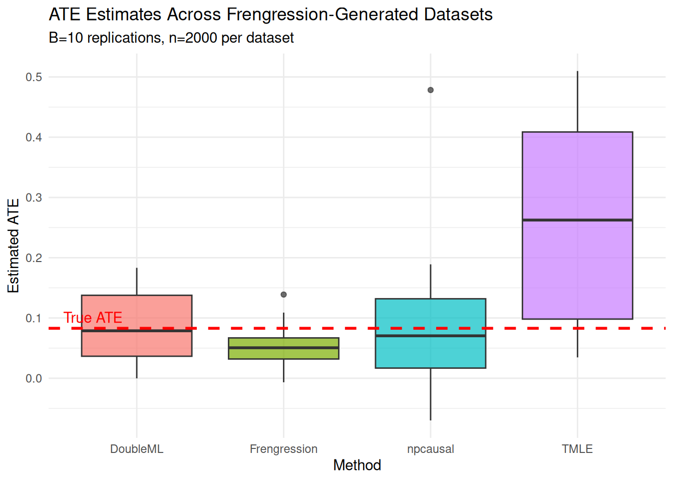
42.8.3 Monte Carlo Benchmarking (LaLonde)
Now do the same exercise with the LaLonde-trained model. Here the confounding structure comes from the real data rather than from my hand-written simulation.
# Compute true ATE empirically from the specified model
y1_lal_true <- predict(model_lal_bench, matrix(1, ncol=1), type="mean", nsample=5000)
y0_lal_true <- predict(model_lal_bench, matrix(0, ncol=1), type="mean", nsample=5000)
true_ate_lal <- as.numeric(y1_lal_true - y0_lal_true)
cat("True ATE (standardized):", round(true_ate_lal, 4), "\n")
True ATE (standardized): 0.2984 True ATE (dollars): 2229 B_lal <- 10
n_syn_lal <- 2000
methods <- c("Frengression", "npcausal", "TMLE", "DoubleML")
ate_mat_lal <- matrix(NA, nrow = B_lal, ncol = length(methods),
dimnames = list(NULL, methods))
se_mat_lal <- ate_mat_lal
cover_mat_lal <- ate_mat_lal
SL.lib_fast <- c("SL.glm.interaction", "SL.ranger", "SL.mean")
set.seed(2024)
for (b in seq_len(B_lal)) {
syn <- sample_joint(model_lal_bench, sample_size = n_syn_lal)
x_syn <- as.numeric(syn$x)
y_syn <- as.numeric(syn$y)
z_syn <- as.data.frame(syn$z)
colnames(z_syn) <- paste0("z", 1:ncol(z_syn))
df_syn <- cbind(data.frame(A = x_syn, Y = y_syn), z_syn)
# --- Frengression ---
tryCatch({
mod_f <- frengression(x_dim = 1, y_dim = 1, z_dim = ncol(z_syn),
x_binary = TRUE, y_binary = FALSE,
noise_dim = 10, hidden_dim = 100, num_layer = 3)
mod_f <- train_y(mod_f, matrix(x_syn, ncol=1), as.matrix(z_syn),
matrix(y_syn, ncol=1),
num_iters = 500, lr = 1e-3, silent = TRUE)
mod_f <- train_xz(mod_f, matrix(x_syn, ncol=1), as.matrix(z_syn),
num_iters = 500, lr = 1e-4, silent = TRUE)
y1_f <- predict(mod_f, matrix(1, ncol=1), type="mean", nsample=1000)
y0_f <- predict(mod_f, matrix(0, ncol=1), type="mean", nsample=1000)
ate_mat_lal[b, "Frengression"] <- y1_f - y0_f
ate_mc <- replicate(100, {
predict(mod_f, matrix(1,ncol=1), type="mean", nsample=200) -
predict(mod_f, matrix(0,ncol=1), type="mean", nsample=200)
})
se_mat_lal[b, "Frengression"] <- sd(ate_mc)
ci_f <- ate_mat_lal[b, "Frengression"] + c(-1,1) * 1.96 * se_mat_lal[b, "Frengression"]
cover_mat_lal[b, "Frengression"] <- (ci_f[1] <= true_ate_lal & true_ate_lal <= ci_f[2])
}, error = function(e) message("Frengression failed on rep ", b, ": ", e$message))
# --- npcausal ---
tryCatch({
fit_np <- ate(y = y_syn, a = x_syn, x = z_syn,
nsplits = 2, sl.lib = SL.lib_fast)
ate_mat_lal[b, "npcausal"] <- fit_np$res$est[3]
se_mat_lal[b, "npcausal"] <- fit_np$res$se[3]
ci <- c(fit_np$res$ci.ll[3], fit_np$res$ci.ul[3])
cover_mat_lal[b, "npcausal"] <- (ci[1] <= true_ate_lal & true_ate_lal <= ci[2])
}, error = function(e) message("npcausal failed on rep ", b, ": ", e$message))
# --- TMLE ---
tryCatch({
fit_tmle <- tmle(Y = y_syn, A = x_syn, W = z_syn, family = "gaussian",
Q.SL.library = SL.lib_fast, g.SL.library = SL.lib_fast)
ate_mat_lal[b, "TMLE"] <- fit_tmle$estimates$ATE$psi
se_mat_lal[b, "TMLE"] <- sqrt(fit_tmle$estimates$ATE$var.psi)
ci_t <- fit_tmle$estimates$ATE$CI
cover_mat_lal[b, "TMLE"] <- (ci_t[1] <= true_ate_lal & true_ate_lal <= ci_t[2])
}, error = function(e) message("TMLE failed on rep ", b, ": ", e$message))
# --- DoubleML ---
tryCatch({
dml_d <- DoubleMLData$new(df_syn, y_col = "Y", d_cols = "A",
x_cols = colnames(z_syn))
lr_l <- lrn("regr.ranger", num.trees = 300, max.depth = 5, min.node.size = 2)
lr_m <- lr_l$clone()
dml_obj <- DoubleMLPLR$new(dml_d, ml_l = lr_l, ml_m = lr_m)
dml_obj$fit()
ate_mat_lal[b, "DoubleML"] <- dml_obj$coef
se_mat_lal[b, "DoubleML"] <- dml_obj$se
ci_d <- c(dml_obj$confint()[1], dml_obj$confint()[2])
cover_mat_lal[b, "DoubleML"] <- (ci_d[1] <= true_ate_lal & true_ate_lal <= ci_d[2])
}, error = function(e) message("DoubleML failed on rep ", b, ": ", e$message))
if (b %% 5 == 0) cat("Completed replication", b, "of", B_lal, "\n")
}Completed replication 5 of 10 Completed replication 10 of 10 bench_lal <- data.frame(
Method = colnames(ate_mat_lal),
Mean_ATE = colMeans(ate_mat_lal, na.rm = TRUE),
Bias = colMeans(ate_mat_lal, na.rm = TRUE) - true_ate_lal,
SD = apply(ate_mat_lal, 2, sd, na.rm = TRUE),
RMSE = sqrt(colMeans((ate_mat_lal - true_ate_lal)^2, na.rm = TRUE)),
Mean_SE = colMeans(se_mat_lal, na.rm = TRUE),
Coverage_95 = colMeans(cover_mat_lal, na.rm = TRUE),
N_valid = colSums(!is.na(ate_mat_lal))
)
kable(bench_lal, digits = 4,
caption = paste0("LaLonde-Based Benchmarking (B=", B_lal,
", n=", n_syn_lal,
", True ATE=", round(true_ate_lal, 4),
" [", round(true_ate_lal * sd(y_lal), 0), " dollars])"))| Method | Mean_ATE | Bias | SD | RMSE | Mean_SE | Coverage_95 | N_valid | |
|---|---|---|---|---|---|---|---|---|
| Frengression | Frengression | 0.2381 | -0.0465 | 0.0911 | 0.0982 | 0.1058 | 0.9 | 10 |
| npcausal | npcausal | -0.0071 | -0.2918 | 0.2307 | 0.3647 | 0.0457 | 0.0 | 10 |
| TMLE | TMLE | 0.3218 | 0.0372 | 0.3674 | 0.3506 | 0.0281 | 0.3 | 10 |
| DoubleML | DoubleML | 0.0371 | -0.2475 | 0.0345 | 0.2496 | 0.0655 | 0.0 | 10 |
ate_long_lal <- as.data.frame(ate_mat_lal) |>
  pivot_longer(everything(), names_to = "Method", values_to = "ATE") |>
  filter(!is.na(ATE))

q_bounds_lal <- quantile(ate_long_lal$ATE, c(0.02, 0.98), na.rm = TRUE)
ate_long_lal_trim <- ate_long_lal |>
  filter(ATE >= q_bounds_lal[1] & ATE <= q_bounds_lal[2])

ggplot(ate_long_lal_trim, aes(x = Method, y = ATE, fill = Method)) +
  geom_boxplot(alpha = 0.7) +
  geom_hline(yintercept = true_ate_lal, linetype = "dashed", color = "red",
             linewidth = 1) +
  annotate("text", x = 0.5, y = true_ate_lal, label = "True ATE",
           hjust = 0, vjust = -0.5, color = "red") +
  labs(title = "ATE Estimates: LaLonde-Based Frengression DGP",
       subtitle = paste0("B=", B_lal, " replications, n=", n_syn_lal,
                         " per dataset (confounding learned from real data)"),
       y = "Estimated ATE (standardized)") +
  theme_minimal() +
  theme(legend.position = "none")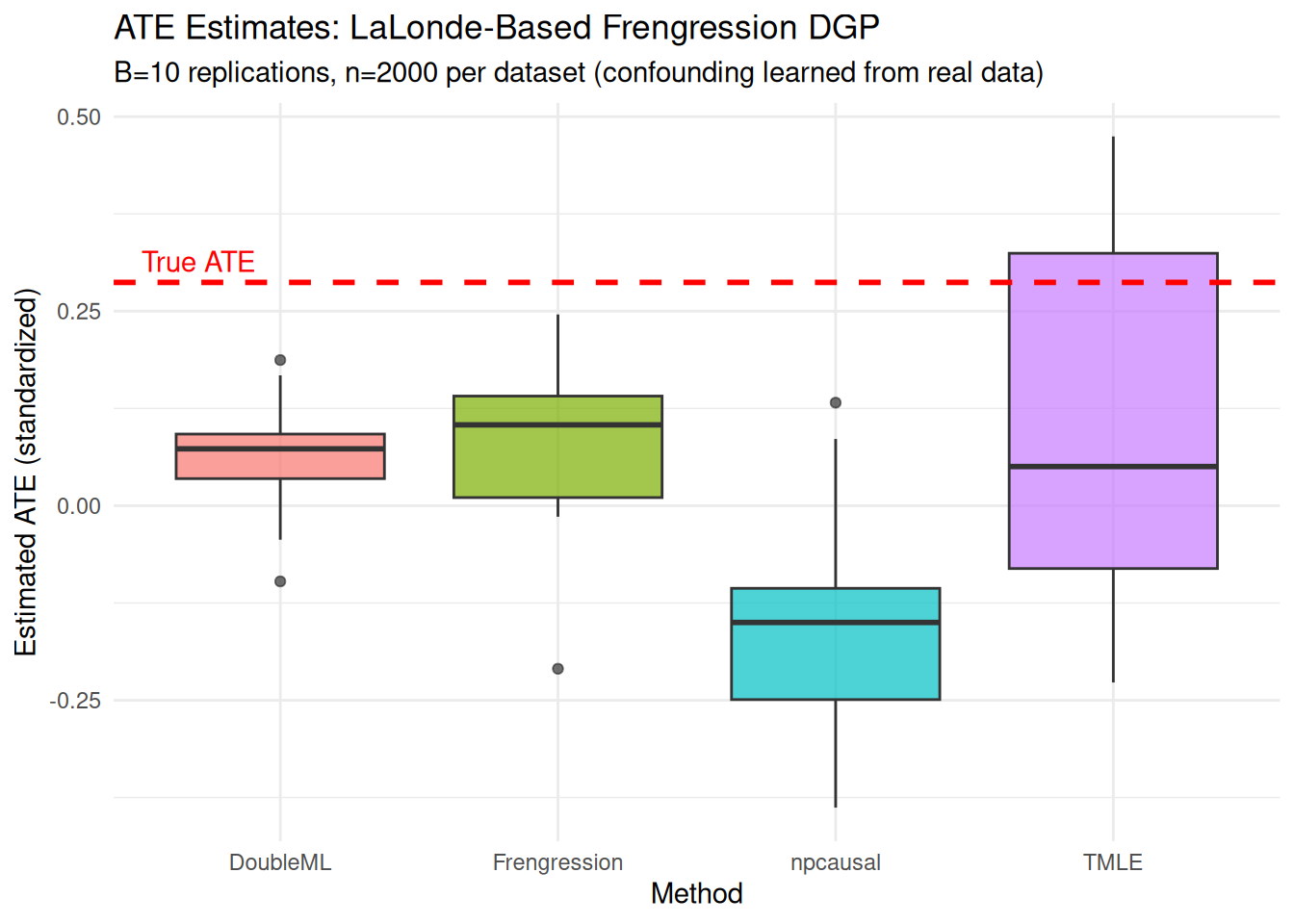
The semiparametric methods show more bias on the LaLonde-generated data than on the hand-written simulation. That is the point of this exercise. The synthetic data has a more realistic propensity surface and prior-earnings distribution, so it is harder than the usual clean simulation.
42.9 Summary
Frengression uses the Evans and Didelez simulation decomposition, but learns the pieces nonparametrically. The practical use is not that it beats TMLE or AIPW for a simple ATE. The practical use is that it can learn a realistic observational distribution, let us impose a known causal effect, and then generate synthetic data where the truth is known.
That makes it useful for benchmarking. The simulation is still artificial, but it is less artificial than writing down a clean logistic model and pretending that it looks like real observational data.
Systematic treatment: Julia.