A common practice is to plot marginal effects with margins and marginsplot, then conclude two effects differ whenever their confidence intervals do not overlap. This can be wrong — overlapping intervals do not imply no significant difference, because the test depends on the joint distribution of the two estimates, not on their marginal distributions separately.
Logistic regression                                     Number of obs = 10,335
                                                        LR chi2(3)    = 353.06
                                                        Prob > chi2   = 0.0000
Log likelihood = -1822.5393                             Pseudo R2     = 0.0883

------------------------------------------------------------------------------
    diabetes | Coefficient  Std. err.      z    P>|z|     [95% conf. interval]
-------------+----------------------------------------------------------------
      female |
     Female  |   1.404111   .4858776     2.89   0.004     .4518088    2.356414
         age |   .0714166   .0063231    11.29   0.000     .0590235    .0838097
             |
female#c.age |
     Female  |  -.0206572   .0078369    -2.64   0.008    -.0360172   -.0052972
             |
       _cons |  -7.041892   .3967299   -17.75   0.000    -7.819468   -6.264315
------------------------------------------------------------------------------


Adjusted predictions                                    Number of obs = 10,335
Model VCE: OIM

Expression: Pr(diabetes), predict()
1._at: age = 20
2._at: age = 30
3._at: age = 40
4._at: age = 50
5._at: age = 60
6._at: age = 70

------------------------------------------------------------------------------
             |            Delta-method
             |     Margin   std. err.      z    P>|z|     [95% conf. interval]
-------------+----------------------------------------------------------------
  _at#female |
     1#Male  |   .0036348   .0009895     3.67   0.000     .0016953    .0055743
   1#Female  |   .0097316   .0018436     5.28   0.000     .0061184    .0133449
     2#Male  |    .007396   .0015622     4.73   0.000     .0043341    .0104579
   2#Female  |   .0160637   .0023434     6.85   0.000     .0114706    .0206568
     3#Male  |   .0149906   .0022831     6.57   0.000     .0105159    .0194653
   3#Female  |    .026406   .0027757     9.51   0.000     .0209657    .0318462
     4#Male  |   .0301469   .0029996    10.05   0.000     .0242677    .0360261
   4#Female  |    .043115   .0030923    13.94   0.000     .0370543    .0491758
     5#Male  |   .0596983   .0040248    14.83   0.000     .0518099    .0675867
   5#Female  |    .069641   .0040284    17.29   0.000     .0617454    .0775366
     6#Male  |   .1147889   .0089467    12.83   0.000     .0972536    .1323242
   6#Female  |   .1106004   .0078699    14.05   0.000     .0951757     .126025
------------------------------------------------------------------------------


Variables that uniquely identify margins: age female

file marginsplot1.svg saved as SVG format


Contrasts of adjusted predictions                       Number of obs = 10,335
Model VCE: OIM

Expression: Pr(diabetes), predict()
1._at: age = 20
2._at: age = 30
3._at: age = 40
4._at: age = 50
5._at: age = 60
6._at: age = 70

-------------------------------------------------------
                    |         df        chi2     P>chi2
--------------------+----------------------------------
         female@_at |
(Female vs Male) 1  |          1        8.49     0.0036
(Female vs Male) 2  |          1        9.47     0.0021
(Female vs Male) 3  |          1       10.09     0.0015
(Female vs Male) 4  |          1        9.06     0.0026
(Female vs Male) 5  |          1        3.05     0.0808
(Female vs Male) 6  |          1        0.12     0.7252
             Joint  |          4       40.48     0.0000
-------------------------------------------------------

---------------------------------------------------------------------
                    |            Delta-method
                    |   Contrast   std. err.     [95% conf. interval]
--------------------+------------------------------------------------
         female@_at |
(Female vs Male) 1  |   .0060969   .0020923      .0019959    .0101978
(Female vs Male) 2  |   .0086677   .0028164      .0031476    .0141878
(Female vs Male) 3  |   .0114154    .003594      .0043712    .0184595
(Female vs Male) 4  |   .0129682   .0043081      .0045244    .0214119
(Female vs Male) 5  |   .0099427   .0056945     -.0012183    .0211037
(Female vs Male) 6  |  -.0041885   .0119155     -.0275425    .0191654
---------------------------------------------------------------------


Variables that uniquely identify margins: age

file marginsplot2.svg saved as SVG format
We fit a logit of diabetes on female, age, and their interaction, on 10,335 NHANES II respondents. The interaction is \(-0.0207\) with a standard error of 0.0078, so the female-male gap narrows with age. The first margins call gives predicted probabilities by gender; the second (with r.female) gives the female-vs-male contrast at each age. (On the general question of marginal effects in nonlinear models, see the previous chapter — the coefficient on the link scale is usually more interpretable.)
Those contrasts run \(.0061\), \(.0087\), \(.0114\), \(.0130\), \(.0099\) and \(-.0042\) at ages 20 through 70, significant through age 50 and not thereafter — the gap widens, peaks in middle age, then closes and reverses sign.
Now the point of the chapter. The female effect at age 20 is \(.0061\) with a 95% interval of \([.0020, .0102]\), and at age 30 it is \(.0087\) with an interval of \([.0031, .0142]\). Those intervals overlap across most of their length. It is tempting to conclude the two effects are not significantly different, but that conclusion does not follow. For two effects \(x\) and \(y\) from the same model,
When \(x\) and \(y\) are positively correlated — as they will be, coming from the same fit — the variance of their difference can be much smaller than either individual variance. So the difference can be significant even when the individual intervals overlap.
Logistic regression                                     Number of obs = 10,335
                                                        LR chi2(3)    = 353.06
                                                        Prob > chi2   = 0.0000
Log likelihood = -1822.5393                             Pseudo R2     = 0.0883

------------------------------------------------------------------------------
    diabetes | Coefficient  Std. err.      z    P>|z|     [95% conf. interval]
-------------+----------------------------------------------------------------
      female |
     Female  |   1.404111   .4858776     2.89   0.004     .4518088    2.356414
         age |   .0714166   .0063231    11.29   0.000     .0590235    .0838097
             |
female#c.age |
     Female  |  -.0206572   .0078369    -2.64   0.008    -.0360172   -.0052972
             |
       _cons |  -7.041892   .3967299   -17.75   0.000    -7.819468   -6.264315
------------------------------------------------------------------------------


Contrasts of adjusted predictions                       Number of obs = 10,335
Model VCE: OIM

Expression: Pr(diabetes), predict()
1._at: age = 20
2._at: age = 30
3._at: age = 40
4._at: age = 50
5._at: age = 60
6._at: age = 70

-------------------------------------------------------
                    |         df        chi2     P>chi2
--------------------+----------------------------------
         female@_at |
(Female vs Male) 1  |          1        8.49     0.0036
(Female vs Male) 2  |          1        9.47     0.0021
(Female vs Male) 3  |          1       10.09     0.0015
(Female vs Male) 4  |          1        9.06     0.0026
(Female vs Male) 5  |          1        3.05     0.0808
(Female vs Male) 6  |          1        0.12     0.7252
             Joint  |          4       40.48     0.0000
-------------------------------------------------------

---------------------------------------------------------------------
                    |            Delta-method
                    |   Contrast   std. err.     [95% conf. interval]
--------------------+------------------------------------------------
         female@_at |
(Female vs Male) 1  |   .0060969   .0020923      .0019959    .0101978
(Female vs Male) 2  |   .0086677   .0028164      .0031476    .0141878
(Female vs Male) 3  |   .0114154    .003594      .0043712    .0184595
(Female vs Male) 4  |   .0129682   .0043081      .0045244    .0214119
(Female vs Male) 5  |   .0099427   .0056945     -.0012183    .0211037
(Female vs Male) 6  |  -.0041885   .0119155     -.0275425    .0191654
---------------------------------------------------------------------


 ( 1)  - r1vs0.female@1bn._at + r1vs0.female@2._at = 0

------------------------------------------------------------------------------
             | Coefficient  Std. err.      z    P>|z|     [95% conf. interval]
-------------+----------------------------------------------------------------
         (1) |   .0025709   .0007946     3.24   0.001     .0010134    .0041283
------------------------------------------------------------------------------
The test gives a difference of \(.0025709\) with a standard error of \(.0007946\), \(z = 3.24\) and \(p = 0.001\). The two effects are different, despite intervals that overlap heavily.
The standard error is what makes the point. Each individual contrast carries a standard error of \(.0021\) and \(.0028\), but their difference carries only \(.00079\) — smaller than either. Solving \(\text{Var}(x-y) = \text{Var}(x) + \text{Var}(y) - 2\text{Cov}(x,y)\) for the correlation gives about \(0.99\): the two contrasts come from the same fitted model evaluated ten years apart, so they move together almost perfectly, and nearly all of their variance cancels in the difference.
Had we ignored the covariance and used \(\sqrt{\text{Var}(x)+\text{Var}(y)} = .0035\), we would have got \(z = 0.73\) and \(p = 0.46\). Same data, same two numbers, opposite conclusion. That is the cost of reading overlap off a graph.
We can do this with native Stata syntax: margins ..., post posts the estimated contrasts as if they were regular coefficients (named r1vs0.female@1._at, r1vs0.female@2._at, etc. — check matrix list e(b) to see the exact names), so lincom can test any linear combination of them natively, without depending on a user-written command.
margins can compute these differences directly with contrast(atcontrast(r)), which compares each evaluation point to the reference:
Logistic regression                                     Number of obs = 10,335
                                                        LR chi2(3)    = 353.06
                                                        Prob > chi2   = 0.0000
Log likelihood = -1822.5393                             Pseudo R2     = 0.0883

------------------------------------------------------------------------------
    diabetes | Coefficient  Std. err.      z    P>|z|     [95% conf. interval]
-------------+----------------------------------------------------------------
      female |
     Female  |   1.404111   .4858776     2.89   0.004     .4518088    2.356414
         age |   .0714166   .0063231    11.29   0.000     .0590235    .0838097
             |
female#c.age |
     Female  |  -.0206572   .0078369    -2.64   0.008    -.0360172   -.0052972
             |
       _cons |  -7.041892   .3967299   -17.75   0.000    -7.819468   -6.264315
------------------------------------------------------------------------------


Contrasts of adjusted predictions                       Number of obs = 10,335
Model VCE: OIM

Expression: Pr(diabetes), predict()
1._at: age = 20
2._at: age = 30
3._at: age = 40
4._at: age = 50
5._at: age = 60
6._at: age = 70

--------------------------------------------------------------
                           |         df        chi2     P>chi2
---------------------------+----------------------------------
                _at#female |
(2 vs 1) (Female vs Male)  |          1       10.47     0.0012
(3 vs 1) (Female vs Male)  |          1        9.28     0.0023
(4 vs 1) (Female vs Male)  |          1        5.48     0.0192
(5 vs 1) (Female vs Male)  |          1        0.50     0.4807
(6 vs 1) (Female vs Male)  |          1        0.65     0.4203
                    Joint  |          4       20.04     0.0005
--------------------------------------------------------------

----------------------------------------------------------------------------
                           |            Delta-method
                           |   Contrast   std. err.     [95% conf. interval]
---------------------------+------------------------------------------------
                _at#female |
(2 vs 1) (Female vs Male)  |   .0025709   .0007946      .0010134    .0041283
(3 vs 1) (Female vs Male)  |   .0053185    .001746      .0018964    .0087407
(4 vs 1) (Female vs Male)  |   .0068713   .0029351      .0011187    .0126239
(5 vs 1) (Female vs Male)  |   .0038458   .0054532     -.0068422    .0145339
(6 vs 1) (Female vs Male)  |  -.0102854   .0127614     -.0352972    .0147264
----------------------------------------------------------------------------


Variables that uniquely identify margins: age

file marginsplot3.svg saved as SVG format
From this we see the difference of effects between point 2 and 1 is .0026, with \(\chi^2(1) = 10.47\) and \(p = 0.0012\) — the same conclusion the lincom test gave above, and indeed the same test: \(3.24^2 = 10.5\). The remaining rows compare each later age to age 20, and the widening gap is significant through age 50 ((4 vs 1): \(\chi^2 = 5.48\), \(p = 0.019\)) before losing precision.
6.2 Summary
Overlapping confidence intervals do not mean two estimates are statistically indistinguishable. A test of the difference depends on the variance of the difference, \(\text{Var}(x-y) = \text{Var}(x) + \text{Var}(y) - 2\,\text{Cov}(x,y)\), and the covariance is nowhere to be seen in a plot of the two intervals separately. Estimates read off the same fitted model at nearby covariate values are strongly positively correlated — 0.99 in this example — so most of their variance cancels in the difference, and the difference is pinned down far more precisely than either level is. The eyeball test is therefore conservative in a specific and misleading way: it reports no difference where a proper test finds one.
The chapter’s numbers make the size of the error concrete. The female-vs-male contrasts at ages 20 and 30 have intervals overlapping across most of their length, yet their difference is 0.0026 with a standard error of 0.00079, \(z = 3.24\), \(p = 0.001\). Ignoring the covariance and combining the two standard errors as \(\sqrt{\text{Var}(x) + \text{Var}(y)}\) would give \(z = 0.73\) and \(p = 0.46\) — same data, opposite conclusion.
So do not read differences off a marginsplot. Ask for them directly:
margins r.varname returns a contrast rather than two levels, with the covariance already handled.
margins ..., contrast(atcontrast(r)) compares every evaluation point to the reference in one call, which is what produced the last table above.
margins ..., post followed by lincom or test handles any single contrast you can write down, using only built-in commands.
The plot is still the right tool for showing how an effect moves across a covariate. It is the wrong tool for judging whether two points on it differ.
Source Code
---title: "Comparing Marginal effects with margins command"date: "2019-04-22"---## Comparing marginal effectsA common practice is to plot marginal effects with `margins` and `marginsplot`, then conclude two effects differ whenever their confidence intervals do not overlap. This can be wrong — overlapping intervals do not imply no significant difference, because the test depends on the joint distribution of the two estimates, not on their marginal distributions separately.```{r}#| echo: false#| message: falselibrary(Statamarkdown)``````{stata}*| cache: truewebuse nhanes2f, clearlogit diabetes i.female##c.age, nologmargins female, at(age=(20 30 40 50 60 70)) marginsplotgraph export "marginsplot1.svg", as(svg) replacemargins r.female, at(age=(20 30 40 50 60 70)) marginsplotgraph export "marginsplot2.svg", as(svg) replace```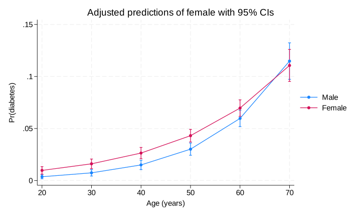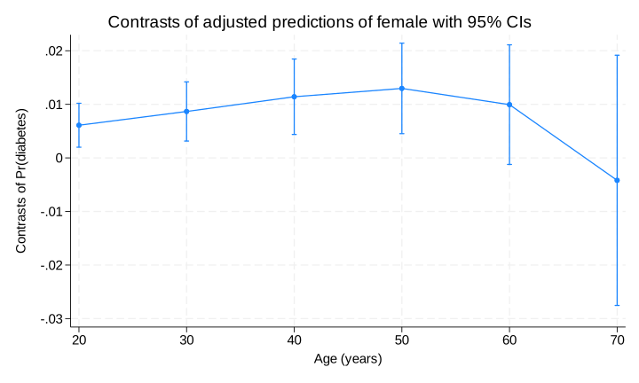We fit a logit of diabetes on female, age, and their interaction, on 10,335 NHANES II respondents. The interaction is $-0.0207$ with a standard error of 0.0078, so the female-male gap narrows with age. The first `margins` call gives predicted probabilities by gender; the second (with `r.female`) gives the female-vs-male contrast at each age. (On the general question of marginal effects in nonlinear models, see the previous chapter — the coefficient on the link scale is usually more interpretable.)Those contrasts run $.0061$, $.0087$, $.0114$, $.0130$, $.0099$ and $-.0042$ atages 20 through 70, significant through age 50 and not thereafter — the gapwidens, peaks in middle age, then closes and reverses sign.Now the point of the chapter. The female effect at age 20 is $.0061$ with a 95%interval of $[.0020, .0102]$, and at age 30 it is $.0087$ with an interval of$[.0031, .0142]$. Those intervals overlap across most of their length. It istempting to conclude the two effects are not significantly different, but that conclusion does not follow. For two effects $x$ and $y$ from the same model,$$ \text{Var}(x - y) = \text{Var}(x) + \text{Var}(y) - 2\,\text{Cov}(x, y). $$ {#eq-comparing-margins-1}When $x$ and $y$ are positively correlated — as they will be, coming from the same fit — the variance of their difference can be much smaller than either individual variance. So the difference can be significant even when the individual intervals overlap.```{stata}*| cache: truewebuse nhanes2f, clearlogit diabetes i.female##c.age, nologmargins r.female, at(age=(20 30 40 50 60 70)) postlincom _b[r1vs0.female@2._at] - _b[r1vs0.female@1._at]```The test gives a difference of $.0025709$ with a standard error of $.0007946$,$z = 3.24$ and $p = 0.001$. The two effects are different, despite intervalsthat overlap heavily.The standard error is what makes the point. Each individual contrast carries astandard error of $.0021$ and $.0028$, but their *difference* carries only$.00079$ — smaller than either. Solving$\text{Var}(x-y) = \text{Var}(x) + \text{Var}(y) - 2\text{Cov}(x,y)$ for thecorrelation gives about $0.99$: the two contrasts come from the same fittedmodel evaluated ten years apart, so they move together almost perfectly, andnearly all of their variance cancels in the difference.Had we ignored the covariance and used$\sqrt{\text{Var}(x)+\text{Var}(y)} = .0035$, we would have got $z = 0.73$ and$p = 0.46$. Same data, same two numbers, opposite conclusion. That is the costof reading overlap off a graph.We can do this with native Stata syntax: `margins ..., post` posts the estimated contrasts as if they were regular coefficients (named `r1vs0.female@1._at`, `r1vs0.female@2._at`, etc. — check `matrix list e(b)` to see the exact names), so `lincom` can test any linear combination of them natively, without depending on a user-written command.`margins` can compute these differences directly with `contrast(atcontrast(r))`, which compares each evaluation point to the reference:```{stata}*| cache: truewebuse nhanes2f, clearlogit diabetes i.female##c.age, nologmargins r.female, at(age=(20 30 40 50 60 70)) contrast(atcontrast(r))marginsplotgraph export "marginsplot3.svg", as(svg) replace```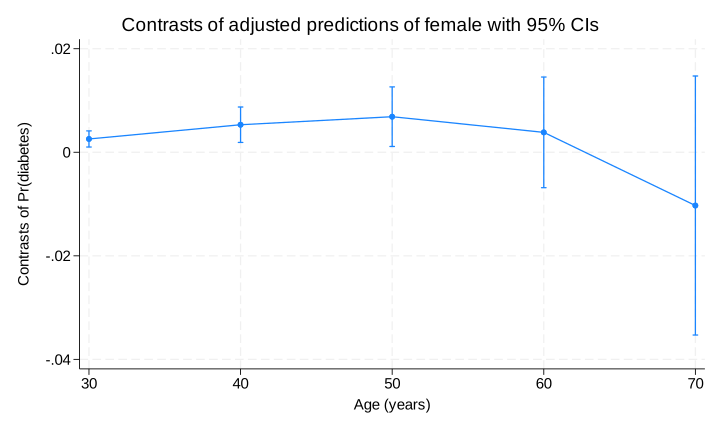From this we see the difference of effects between point 2 and 1 is .0026, with$\chi^2(1) = 10.47$ and $p = 0.0012$ — the same conclusion the `lincom` testgave above, and indeed the same test: $3.24^2 = 10.5$. The remaining rows compareeach later age to age 20, and the widening gap is significant through age 50((4 vs 1): $\chi^2 = 5.48$, $p = 0.019$) before losing precision.## SummaryOverlapping confidence intervals do not mean two estimates are statisticallyindistinguishable. A test of the difference depends on the variance of thedifference,$\text{Var}(x-y) = \text{Var}(x) + \text{Var}(y) - 2\,\text{Cov}(x,y)$,and the covariance is nowhere to be seen in a plot of the two intervalsseparately. Estimates read off the same fitted model at nearby covariate valuesare strongly positively correlated — 0.99 in this example — so most of theirvariance cancels in the difference, and the difference is pinned down far moreprecisely than either level is. The eyeball test is therefore conservative in aspecific and misleading way: it reports no difference where a proper test findsone.The chapter's numbers make the size of the error concrete. The female-vs-malecontrasts at ages 20 and 30 have intervals overlapping across most of theirlength, yet their difference is 0.0026 with a standard error of 0.00079,$z = 3.24$, $p = 0.001$. Ignoring the covariance and combining the two standarderrors as $\sqrt{\text{Var}(x) + \text{Var}(y)}$ would give $z = 0.73$ and$p = 0.46$ — same data, opposite conclusion.So do not read differences off a `marginsplot`. Ask for them directly:- `margins r.varname` returns a contrast rather than two levels, with the covariance already handled.- `margins ..., contrast(atcontrast(r))` compares every evaluation point to the reference in one call, which is what produced the last table above.- `margins ..., post` followed by `lincom` or `test` handles any single contrast you can write down, using only built-in commands.The plot is still the right tool for showing how an effect moves across acovariate. It is the wrong tool for judging whether two points on it differ.


