---
title: "Synthetic Control in R and Stata"
date: "2021-09-12"
---
## Synthetic control
Abadie et al. have a few papers on synthetic control --- Abadie, Diamond and
Hainmueller ([2010](https://doi.org/10.1198/jasa.2009.ap08746), *JASA*) and
([2015](https://doi.org/10.1111/ajps.12116), *AJPS*), and Abadie's
([2021](https://doi.org/10.1257/jel.20191450), *JEL*) survey. The key idea is for a case study situation. A single unit, say a state/firm/country is exposed to a shock, and we are interested in the effect of that shock. For example, Card and Krueger (1994) studied the effect of a minimum wage increase in New Jersey. They used diff-in-diff, with Pennsylvania as the control state. The point of synthetic control is that maybe parallel trend assumption does not hold for the control unit. Is Pennsylvania a good control for New Jersey? Does it follow the same trend as New Jersey? Maybe not. Synthetic control is to generate a more comparable control with some combination of multiple control units, which can have a much closer parallel trend as the treated unit, than using any of the control units.
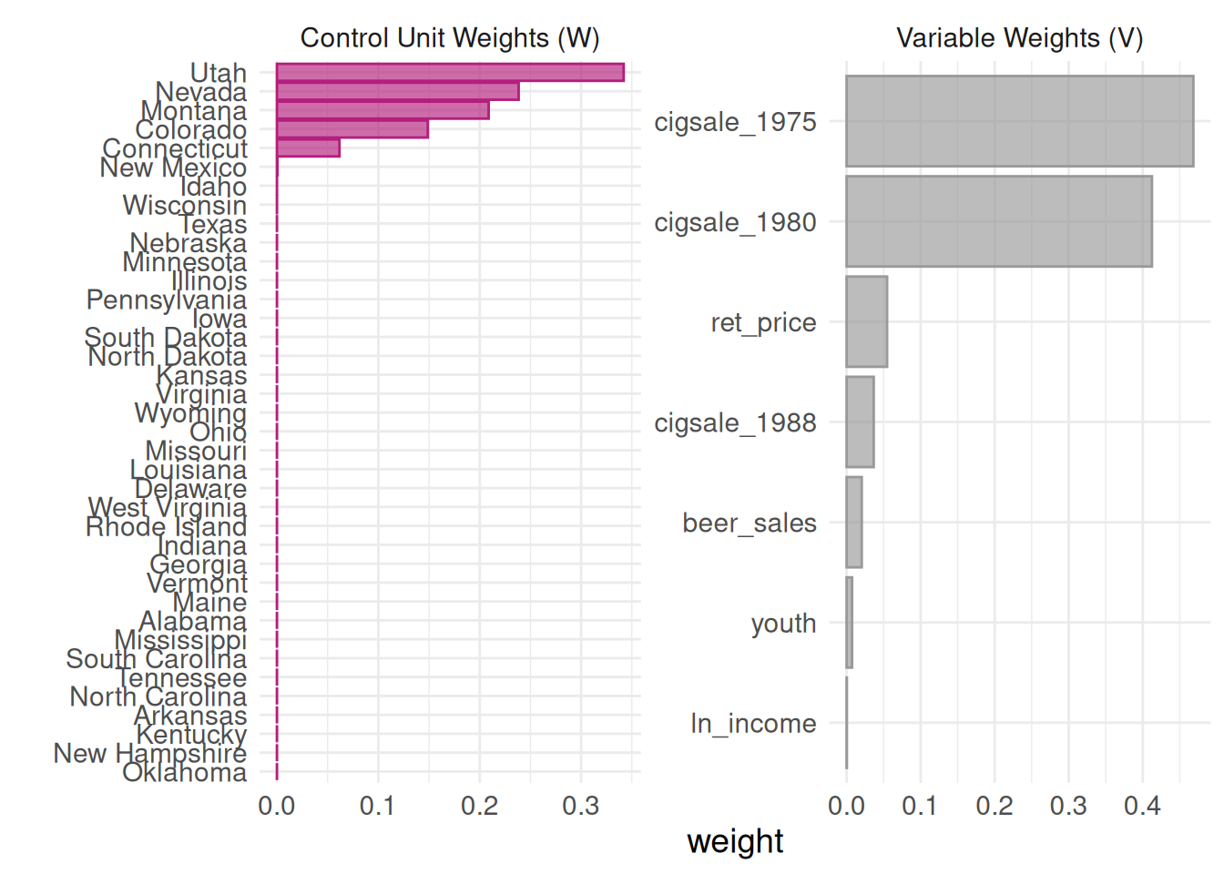
Now, how to construct this synthetic control unit? Basically it is a weighted average of multiple control units. There are two sets of weights to be determined. One set for the control units, one set to determine the importance of predictors. Abadie et al (2010) propose to choose a set of $w_i$'s so that the resulting synthetic control best resembles the pre-intervention values for the treated unit of predictors of the outcome variable, subject to the constraints that the weights are non-negative and sum to 1. Another set of weights $v_h$ for predictor importance is determined such that it minimizes the mean squared prediction error (MSPE) of this synthetic control with respect to the outcome in the pre-treatment period. The intuition of these weights are to pick $w_i$'s to make the weighted sum of each predictor as close to the treated unit's value of predictor as close as possible, given a set of $v_h$'s. Then $v_h$'s are determined by how important each predictor is to predict the outcome. We don't use any information post-treatment to determine the weights. But we can use pre-treatment outcome to see the relative importance of each predictor in terms of predictor outcome. We can do this by out-of-sample validation. Basically divide the pre-treatment period into training and validation periods (that's one reason that the pre-treatment period cannot be too short). Iterate the process of choosing $w_i$ and $v_h$ to achieve a minimization of MSPE in the validation period.
## inference
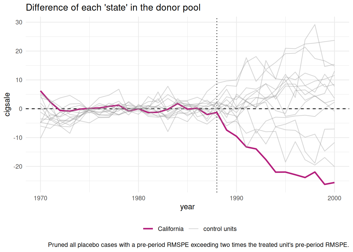
Since synthetic control is for case study situation, we have essentially one treated unit and one synthetic control. The usual inference method would not work. Abadie et al suggested a permutation based approach. The basic idea is to permute the label of treatment; in other words, suppose one control unit is now a treated unit. Then follow the same procedure to get the synthetic control for that "treated unit"; look at the effect. Now if the treatment is truly for the treated unit only, then there would not be any effect for all the control unit. Therefore we can have a distribution of treatment effects after permutation of treatment label.
## an example
The canonical synthetic control is implemented in both R and Stata (the `Synth` package, [CRAN](https://cran.r-project.org/package=Synth); see Abadie, Diamond and Hainmueller's [*JSS* paper](https://www.jstatsoft.org/article/view/v042i13) for the software description). We use a package called "tidysynth" here to study one of the original examples, which evaluates the impact of Proposition 99 on cigarette consumption in California.
```{r}
#| label: rchunk1
#| echo: true
#| cache: true
library(tidysynth)
library(dplyr)
library(tidyverse)
library(ggplot2)
library(tidyr)
data("smoking")
smoking %>% dplyr::glimpse()
```
The panel is 1,209 state-years: 39 states from 1970 to 2000, with per-capita
cigarette sales in packs as the outcome and log income, beer sales, the share
aged 15–24, and retail price as predictors. California passed Proposition 99 in
1988, so there are 19 pre-treatment years to fit the weights and 12
post-treatment years to measure the effect.
```{r}
#| label: rchunk2
#| echo: true
#| cache: true
smoking_out <-
    smoking %>%
    # initial the synthetic control object
    synthetic_control(outcome = cigsale, # outcome
                    unit = state, # unit index in the panel data
                    time = year, # time index in the panel data
                    i_unit = "California", # unit where the intervention occurred
                    i_time = 1988, # time period when the intervention occurred
                    generate_placebos=T # generate placebo synthetic controls (for inference)
                    ) %>%
    # Generate the aggregate predictors used to fit the weights
    # average log income, retail price of cigarettes, and proportion of the
    # population between 15 and 24 years of age from 1980 - 1988
  generate_predictor(time_window = 1980:1988,
                     ln_income = mean(lnincome, na.rm = T),
                     ret_price = mean(retprice, na.rm = T),
                     youth = mean(age15to24, na.rm = T)) %>%
    # average beer consumption in the donor pool from 1984 - 1988
  generate_predictor(time_window = 1984:1988,
                     beer_sales = mean(beer, na.rm = T)) %>%
    # Lagged cigarette sales
  generate_predictor(time_window = 1975,
                     cigsale_1975 = cigsale) %>%
  generate_predictor(time_window = 1980,
                     cigsale_1980 = cigsale) %>%
  generate_predictor(time_window = 1988,
                     cigsale_1988 = cigsale) %>%
    # Generate the fitted weights for the synthetic control
  generate_weights(optimization_window = 1970:1988, # time to use in the optimization task
                   margin_ipop = .02,sigf_ipop = 7,bound_ipop = 6 # optimizer options
  ) %>%
  # Generate the synthetic control
  generate_control()

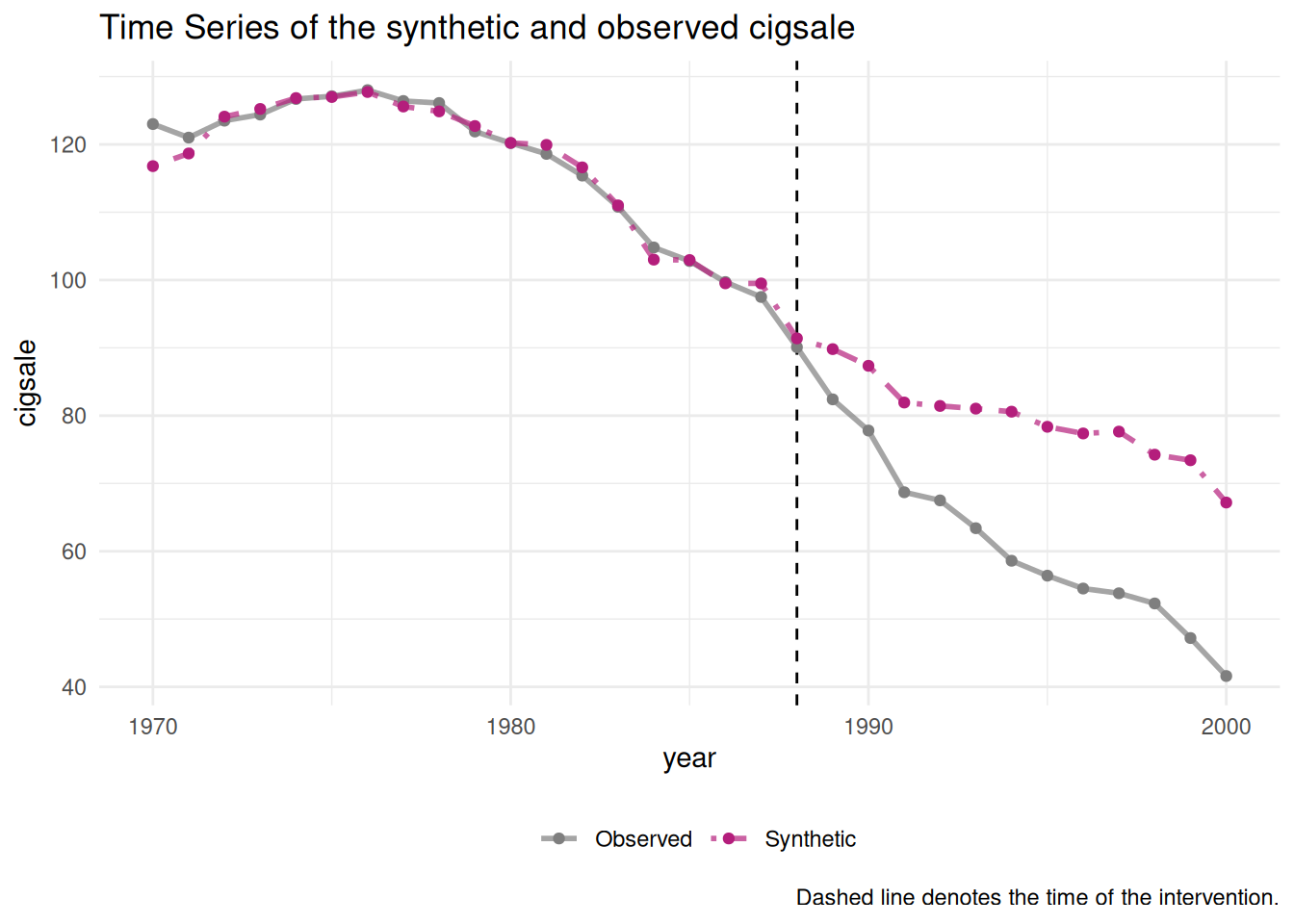
smoking_out %>% plot_trends()
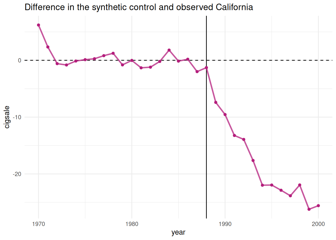
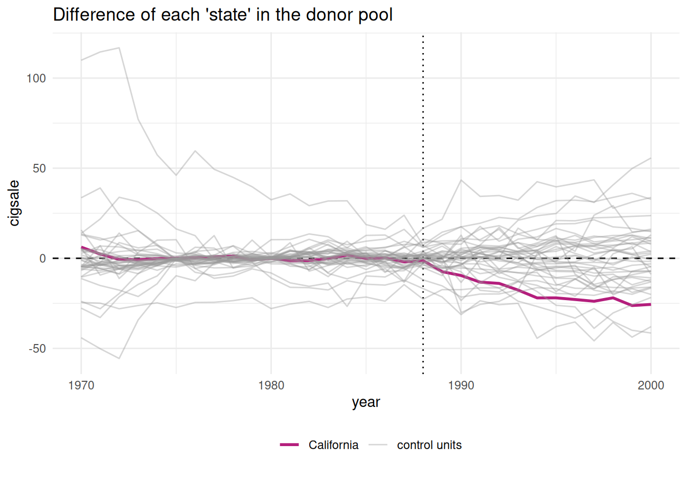
smoking_out %>% plot_differences()
smoking_out %>% plot_weights()
smoking_out %>% grab_balance_table()
smoking_out %>% plot_placebos()
smoking_out %>% plot_placebos(prune = FALSE)
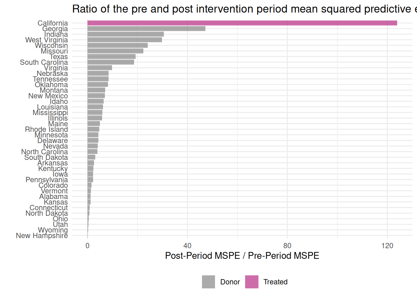
smoking_out %>% plot_mspe_ratio()
smoking_out %>% grab_significance()
smoking_out %>% grab_synthetic_control()
smoking_out %>% grab_synthetic_control(placebo = T)
smoking_out %>%
  tidyr::unnest(cols = c(.outcome))
```
The balance table is where to judge whether the synthetic control is worth
trusting, and it does well. Retail price matches to three digits (89.4 against
89.4), the youth share to 0.174 against 0.174, beer sales 24.3 against 24.2. The
pre-treatment outcomes match closely too: 1975 cigarette sales 127 against 127
and 1980 sales 120 against 120. Compare those with the raw donor-pool averages
in the third column — 137 and 138 — and the value of weighting is obvious. The
one predictor that does not match is log income, 10.1 against 9.85, which the
optimiser evidently judged less important for predicting the outcome.
The 1988 row is the one to read carefully: 90.1 against 91.4. That is the last
pre-treatment year and it is fitted, not predicted, so it is a diagnostic rather
than a result.
Inference comes from the placebo table. California's ratio of post- to
pre-treatment MSPE is 124, the largest of all 39 units — Georgia is next at
47.2, less than half. Being ranked first of 39 gives a Fisher exact $p$ of
$1/39 = 0.0256$. This is a permutation statement, not a sampling one: it says no
untreated state shows a post-1988 divergence from its own synthetic control as
large as California's, relative to how well each was fitted beforehand.
## Generalized Synthetic Control
The idea of generalized SC is to combine both an interactive fixed effect model and synthetic control. It is basically a panel data synthetic control. It naturally takes multiple treated units and uses bootstrap to get standard errors. It generates ATT with standard errors.
Examples are here: <https://yiqingxu.org/packages/gsynth/>
```{r}
#| label: rchunk3
#| echo: true
#| cache: true
## for processing C++ code
require(Rcpp)
## for plotting
require(ggplot2)
require(GGally)
## for parallel computing
require(foreach)
require(future)
require(doParallel)
require(abind)
require(lfe)
library(gsynth)
## ## Syntax has been updated since v.1.2.0.
## ## Comments and suggestions -> yiqingxu@stanford.edu.
data(gsynth)
library(panelView)
## ## See bit.ly/panelview4r for more info.
## ## Report bugs -> yiqingxu@stanford.edu.
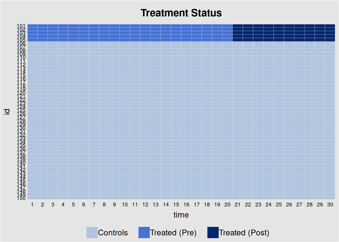
panelview(Y ~ D, data = simdata,  index = c("id","time"), pre.post = TRUE)
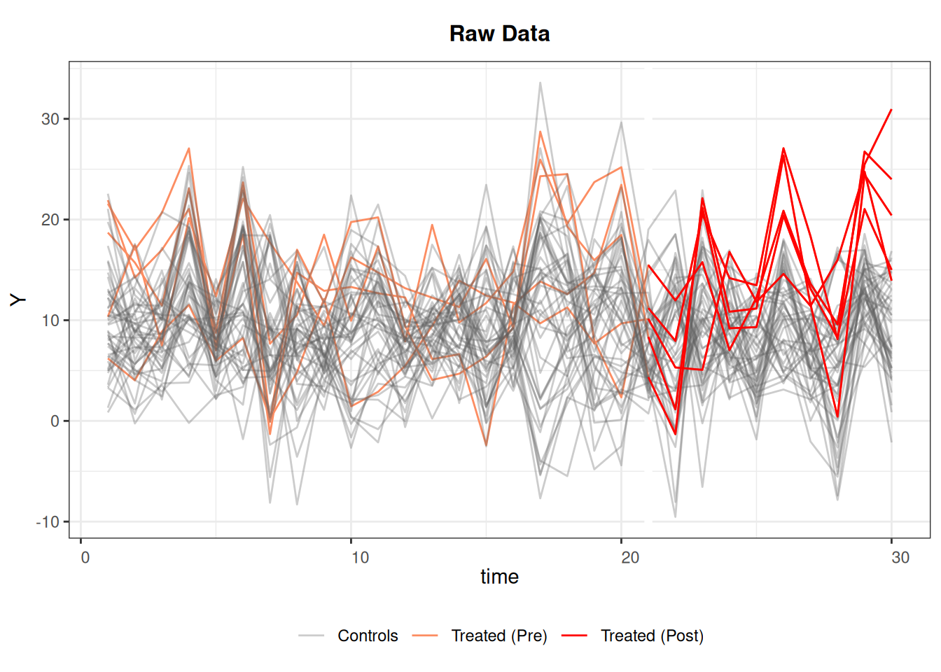
panelview(Y ~ D, data = simdata, index = c("id","time"), type = "outcome")
system.time(
    out <- gsynth(Y ~ D + X1 + X2, data = simdata, index = c("id","time"), force = "two-way", CV = TRUE, r = c(0, 5), se = TRUE, inference = "parametric", nboots = 100, parallel = FALSE)
)
print(out)
out$est.att
out$est.avg
out$est.beta
system.time(
out <- gsynth(Y ~ D + X1 + X2, data = simdata, index = c("id","time"),
    force = "two-way", CV = TRUE, r = c(0, 5), se = TRUE,
    inference = "parametric", nboots = 100, parallel = TRUE, cores = 4)
)
# cumuEff was removed in newer gsynth versions (now a wrapper for fect)
# cumu1 <- cumuEff(out, cumu = TRUE, id = NULL, period = c(0,5))
# cumu1$est.catt

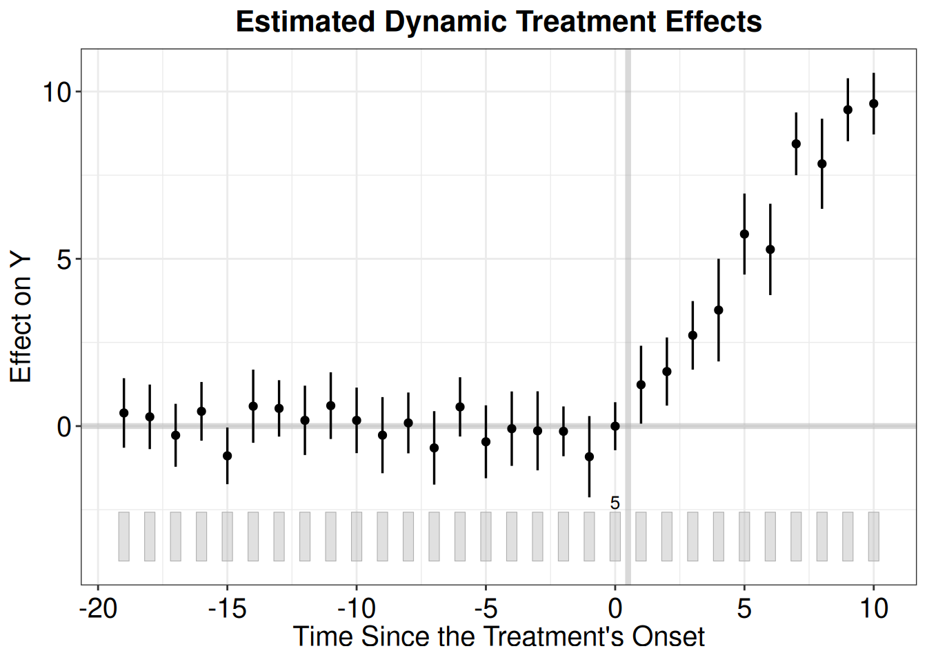
plot(out)
```
`simdata` is gsynth's own simulated panel: 5 treated units and 45 controls over
30 periods, with treatment starting in period 21 for the treated group, an
interactive fixed-effect structure, and two covariates.
The estimated average ATT is 5.084 with a standard error of 0.292 and a 95%
interval of $[4.512, 5.656]$. The covariate coefficients come out at 1.454 for
`X1` and 3.507 for `X2`. The period-by-period table is the part worth reading,
because it includes the pre-treatment periods: those run from $-19$ to $-1$ and
should be centred on zero if the interactive fixed-effect model has absorbed the
common factors. They mostly are — $0.059$, $-0.117$, $-0.890$, $1.295$,
$-1.203$, $2.220$ and so on — bouncing around zero with standard errors of about
0.5 to 0.7. Two of them ($-16$ and $-14$) are individually significant at 5%,
which is roughly what one expects from nineteen independent tests at that level.
---
<!-- see-also-footer -->
*Systematic treatment: [Julia](https://xiangao.github.io/causal_econometrics_julia/synthetic-control-did-tasc.html).*