Code
The longitudinal modified treatment policy (LMTP) framework, developed in epidemiology and biostatistics, handles settings where the standard ATE is poorly defined: continuous or multivalued treatments, time-varying exposures, or hypothetical interventions that would violate positivity. This chapter follows Nicholas Williams.
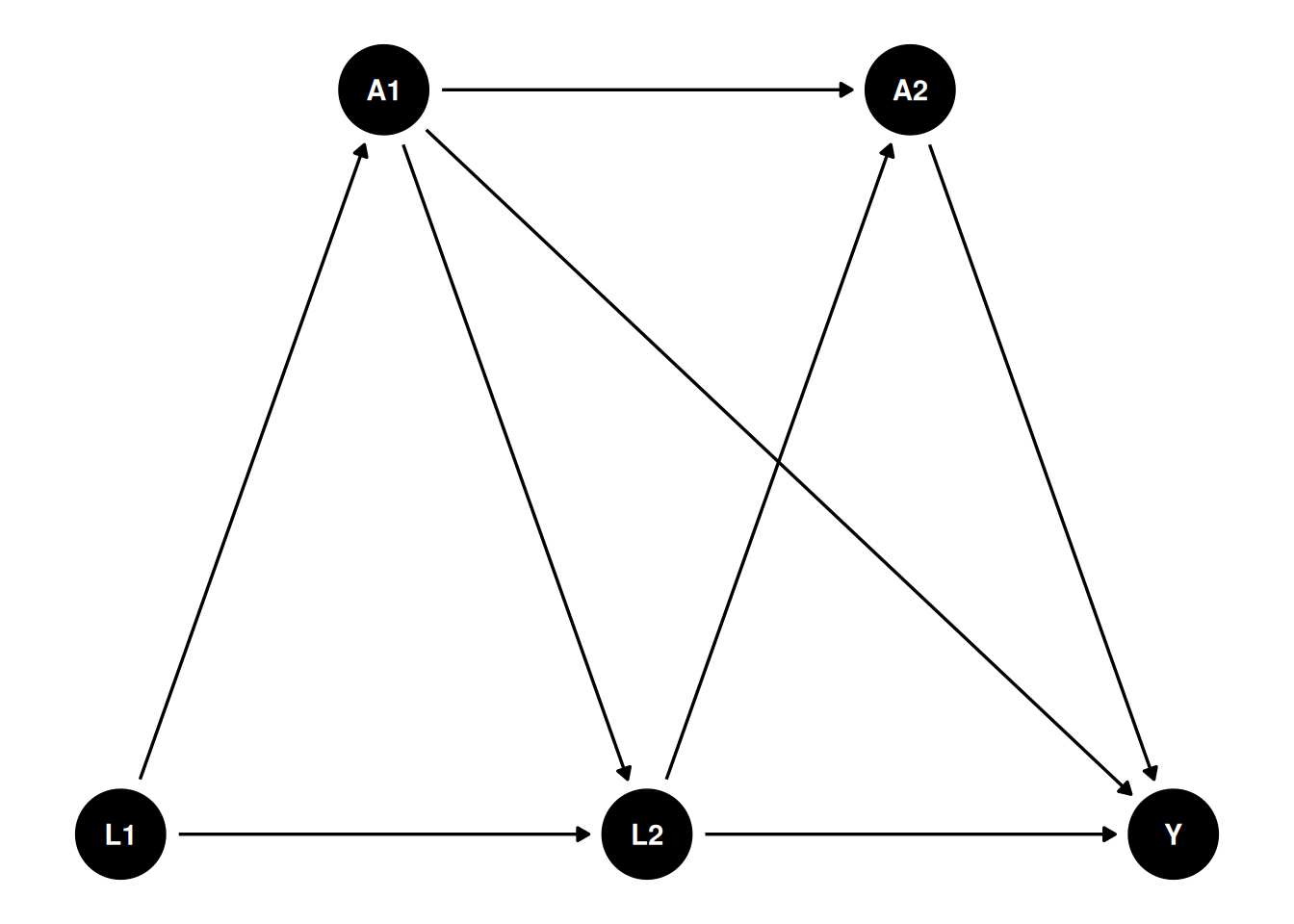
Suppose we have such a DAG:
We have multiple time points, and the treatment \(A\) is time-varying. We are interested in not only the ATE of \(A_2\) on \(Y\), but also some other hypothetical interventions.
Consistency. The observed outcome under the treatment actually received equals the corresponding potential outcome, and the shifted intervention is well defined — no hidden versions of it.
Sequential unconfoundedness. There are no unmeasured confounders of treatment at any time point given the history. The stronger sequential randomization condition conditions on the full history including past natural values of treatment; some estimators need that version and others do not, so it is worth knowing which one a given result assumes.
Positivity, in the form the shift requires. Roughly: if a unit with history \(h_t\) can receive \(a_t\), then the shifted value \(d(a_t, h_t)\) must also have support given \(h_t\). This is where modified treatment policies earn their keep. A static always-treat or never-treat rule can demand support the data does not have, while a bounded shift of the observed treatment stays inside it.
For continuous treatments, a smoothness condition. The influence-function estimators below assume the shift function is piecewise smooth and invertible in \(a_t\), which is what lets the density of the shifted treatment be written in terms of the observed one.
The always-treat and never-treat demonstration below is, on that reading, an unusual lead example for this framework: it is the easiest case to follow, and also the case whose positivity is most likely to fail. A bounded continuous shift is the canonical LMTP application. Díaz et al., https://arxiv.org/abs/2006.01366, state the assumptions precisely.
Some notations commonly used in this literature: We observe \(Z = (L_0, A_0, L_1, A_1, Y)\), where \(L\) is the observed confounder, \(A\) is the treatment, and \(Y\) is the outcome. The treatment \(A\) can be time-varying. We can also have multiple treatments at different time points. For example, we can have \(A_2\), \(A_3\), etc. In this graph, baseline \(L_0\) affects \(A_0\), which in turn affects \(L_1\), which then affects \(A_1\), and finally \(A_1\) affects the outcome \(Y\).
History \(H_t\) is the history of data up to time \(t\), right before \(A_t\). for example, \(H_1 = (L_0, A_0, L_1)\), and \(H_2 = (L_0, A_0, L_1, A_1)\). \(d\) is the hypothetical intervention function, or shift function, which is a function of the history \(H_t\) and the treatment \(A_t\). For example, \(d_0(a_0,h_0,\epsilon_0)\) is a user-given function to map \(a_0\), \(h_0\), and \(\epsilon_0\) to a potential treatment value. The function \(d\) can be deterministic, or it can be stochastic. Then we can replace \(A_0\) with \(A_0^d = d_0(A_0, H_0, \epsilon_0)\). Then after that \(A_1(A_0^d)\) is called the natural value of treatment.
This is very general, comparing to the static treatment regime.
Suppose treatment \(A\) is a function of the history of treatment and confounders, for example, \(A = d(A_1, L_1, A_2, L_2)\). \(A\) can be set to a fixed value, say 1 or 0, or some value \(A^d\). This function \(d\) can be anything, it can be taking a deterministic value, or it can be a function that takes the natural treatment value \(A\) as input. In the package “lmtp”, this is called a shift function, or hypothetical intervention. For example, \(d\) can be set to 1 if \(age < 30\), or \(d\) can be set to double the natural value of \(A\). Many possibilities.
In comparison, for ATE, we only need to set \(A\) to 0 or 1.
Under this LMTP, the causal parameter is
\[ \theta = E[Y^{\bar A^d}] \tag{35.1}\]
\(Y^{\bar A^d}\) is the potential outcome under the hypothetical intervention \(\bar A^d\). At time 1, \(A^d_1 = d(A_1,H_1)\).
A simulated data set makes the estimation concrete.
This simulation is from Susmann et al. (2024) “Longitudinal Generalizations of the Average Treatment Effect on the Treated for Multi-valued and Continuous Treatments”. I modified slightly to fit the DAG above.
library(tidyverse)
library(tidyr)

mtp <- function(data, trt) {
  a <- data[[trt]]
  a * 0 + 1
}
simulate_data <- function(seed, N, tau, sigma = 0.5) {
  set.seed(seed)

  data <- tibble(id = 1:N)

  for(t in 1:tau) {
    Lt <- paste0("L_", t)
    Ltd <- paste0("L_", t, "d")

    At <- paste0("A_", t)
    Atd <- paste0("A_", t, "d")

    Lt1 <- paste0("L_", t - 1)
    Lt1d <- paste0("L_", t - 1, "d")

    At1 <- paste0("A_", t - 1)
    At1d <- paste0("A_", t - 1, "d")

    if(t == 1) {
      data[[Lt]] <- runif(N, 0, 1)
      data[[Ltd]] <- data[[Lt]]

      data[[At]] <- rbinom(N, size = 1, prob = 0.5)
    }
    else {
      # L_t depends on the previous treatment A_{t-1} (the DAG edge A1 -> L2),
      # which is the time-varying confounding this chapter is about.
      data[[Lt]] <- rnorm(N, mean = 0.25 * data[[Lt1]] + 0.4 * data[[At1]], 0.5)
      data[[Ltd]] <- rnorm(N, mean = 0.25 * data[[Lt1d]] + 0.4 * data[[At1d]], 0.5)

      data[[At]] <- rbinom(N, size = 1, prob = plogis(0.5 - 0.2 * data[[At1]] + 0.1 * data[[Lt1]]))
    }

    data[[Atd]] <- mtp(data, At)
  }
  # Y depends on the final treatment A_2 and confounder L_2, and also directly
  # on the first-period treatment A_1 (the DAG edge A1 -> Y).
  data$Y  <- rnorm(N, data[[At]] + data[[Lt]] + 0.5 * data[["A_1"]], sigma)
  data$Yd <- rnorm(N, data[[Atd]] + data[[Ltd]] + 0.5 * data[["A_1d"]], sigma)
  data
}

simulated_data1 <- simulate_data(seed = 123, N = 10000, tau = 2)

mean(simulated_data1$Yd)
[1] 2.028593mtp <- function(data, trt) {
a <- data[[trt]]
a * 0 + 0
}
simulated_data2 <- simulate_data(seed = 123, N = 10000, tau = 2)
mean(simulated_data2$Yd)[1] 0.1285934[1] 1.9Note in this simulation the variables ending with “d” are the variables under hypothetical intervention, or modified treatment policy. \(L_1\) is from \(\text{Uniform}(0,1)\), and \(L_2\) is from \(N(0.25 L_1 + 0.4 A_1,\ 0.5)\) – so the time-varying confounder \(L_2\) depends on the earlier treatment \(A_1\), which is the time-varying confounding this chapter is about. The treatment \(A_1\) is from a Bernoulli distribution with probability 0.5, and the treatment \(A_2\) is from a Bernoulli distribution with probability \(\text{plogis}(0.5 - 0.2 A_1 + 0.1 L_1)\). The outcome \(Y\) is from a normal distribution with mean \(A_2 + L_2 + 0.5 A_1\), so \(Y\) depends on both the current treatment \(A_2\) and the lagged treatment \(A_1\). In the code, the first modified treatment policy sets treatment to 1 in every period (simulated_data1) and the second sets it to 0 in every period (simulated_data2); the reported difference \(E[Y^{d}_{\text{always }1}] - E[Y^{d}_{\text{always }0}]\) is the effect of the always-treat versus never-treat static regimes.
The always-treat regime gives \(E[Y^d] = 2.029\), never-treat gives 0.129, and their difference is 1.900 — and that 1.9 decomposes exactly into the three routes the DGP contains: 1 from \(A_2\) direct, 0.5 from \(A_1\) direct, and 0.4 through the \(A_1 \to L_2 \to Y\) path, since \(L_2\) shifts by 0.4 and enters \(Y\) with coefficient 1.
In this case, we can just do a linear regression to get the effect of A2 on Y, knowing the exact DAG.
Call:
glm(formula = Y ~ L_2 + A_1 + A_2, data = simulated_data1)

Coefficients:
              Estimate Std. Error t value Pr(>|t|)
(Intercept) -3.453e-05  9.615e-03  -0.004    0.997
L_2          9.998e-01  9.889e-03 101.103   <2e-16 ***
A_1          4.940e-01  1.079e-02  45.779   <2e-16 ***
A_2          1.000e+00  1.027e-02  97.380   <2e-16 ***
---
Signif. codes:  0 '***' 0.001 '**' 0.01 '*' 0.05 '.' 0.1 ' ' 1

(Dispersion parameter for gaussian family taken to be 0.2500364)

    Null deviance: 9257.2  on 9999  degrees of freedom
Residual deviance: 2499.4  on 9996  degrees of freedom
AIC: 14523

Number of Fisher Scoring iterations: 2
Knowing the DAG, the regression recovers every structural coefficient: \(L_2\) at 0.9998, \(A_1\) at 0.4940 and \(A_2\) at 1.0000, against true values of 1, 0.5 and 1. Note this identifies the direct effect of \(A_1\) only; its path through \(L_2\) is blocked by conditioning on \(L_2\), which is why the total of 1.9 above cannot be read off this table.
Now consider a different MTP: set half of the time to 0 and leave the other half unchanged. \[ d(a_t, \epsilon_t) = \begin{cases} 0, & \text{if } \epsilon_t < .5 \ and \ a_t =1 \\ a_t, & \text{otherwise} \end{cases} \tag{35.2}\]
This is, say, to set half of smokers to non-smokers, and the other half remain smokers.
# mtp <- function(data, trt) {
#   a <- data[[trt]]
#   epsilon <- rbinom(nrow(data), size = 1, prob = 0.5)
#   ifelse(epsilon <.5 & a == 1, 0, a)
# }
d <- function(a) {
  epsilon <- runif(length(a))
  ifelse(epsilon < 0.5 & a == 1, 0, a)
}
simulated_data1$m3_d <- simulated_data1$Y

m2 <- glm(m3_d ~ L_1 + A_1 + L_2 + A_2, data = simulated_data1)
summary(m2)
Call:
glm(formula = m3_d ~ L_1 + A_1 + L_2 + A_2, data = simulated_data1)

Coefficients:
             Estimate Std. Error t value Pr(>|t|)
(Intercept) -0.005815   0.012842  -0.453    0.651
L_1          0.011964   0.017621   0.679    0.497
A_1          0.494512   0.010814  45.729   <2e-16 ***
L_2          0.998831   0.009987 100.015   <2e-16 ***
A_2          0.999873   0.010273  97.334   <2e-16 ***
---
Signif. codes:  0 '***' 0.001 '**' 0.01 '*' 0.05 '.' 0.1 ' ' 1

(Dispersion parameter for gaussian family taken to be 0.2500499)

    Null deviance: 9257.2  on 9999  degrees of freedom
Residual deviance: 2499.2  on 9995  degrees of freedom
AIC: 14525

Number of Fisher Scoring iterations: 2
Call:
glm(formula = m2_d ~ L_1 + A_1, data = simulated_data1)

Coefficients:
            Estimate Std. Error t value Pr(>|t|)
(Intercept)  0.30716    0.01531   20.07   <2e-16 ***
L_1          0.26079    0.02384   10.94   <2e-16 ***
A_1          0.87604    0.01367   64.08   <2e-16 ***
---
Signif. codes:  0 '***' 0.001 '**' 0.01 '*' 0.05 '.' 0.1 ' ' 1

(Dispersion parameter for gaussian family taken to be 0.4669449)

    Null deviance: 6633.7  on 9999  degrees of freedom
Residual deviance: 4668.0  on 9997  degrees of freedom
AIC: 20768

Number of Fisher Scoring iterations: 2[1] 0.6518997The recursion makes the blocked path visible. The first regression, on the full history, again gives \(A_1 = 0.4945\) — the direct effect. The second, after substituting the shifted \(A_2\) and regressing on \(L_1\) and \(A_1\) only, gives \(A_1 = 0.8760\), which is close to the total \(0.5 + 0.4 = 0.9\): dropping \(L_2\) from the conditioning set lets \(A_1\)’s indirect path back in. The final average is 0.652, the expected outcome under the stochastic half-off regime, sitting between the always-treat 2.029 and never-treat 0.129 as it should.
Note this recursive process is based on Diaz, et al. (2023) “Nonparametric Causal Effects Based on Longitudinal Modified Treatment Policies”.
Here is how exactly we estimate it: we start with the last time point. Regress it on previous treatment and confounders, and then get the predicted value with \(A\) changed based on the MTP. Regress that predicted value on the previous treatment and confounders, get predicted values with \(A\) changed based on MTP. Repeat until the first time point. The average of the predicted value at time 1 is the expected value under this MTP.
The shift function d() above is a stochastic intervention: at each call it draws a fresh \(\epsilon \sim \text{Uniform}(0,1)\) and, with probability 0.5, switches a treated unit (\(a=1\)) to \(0\), otherwise leaves \(a\) unchanged. The regime is “at each time point, draw independently conditional on history and apply this rule”; because the draw is independent across time points and units, calling d() separately for \(A_2\) and \(A_1\) is what implements that regime. (By contrast, the d1/d2 functions used with lmtp_tmle below are deterministic static regimes – always 1 and always 0.)
This is basically g-formula extended to longitudinal data.
In a general case, this is the generalized g-formula to estimate \(\theta\):
Set \(m_{\tau + 1} = Y\), let \(A_t^d = d(A_t, H_t)\). For \(t = \tau, \ldots, 1\), recursively define:
\[ m_t(a_t, h_t) = E[m_{t + 1} (A_{t+1}^d, H_{t+1}) | A_t = a_t, H_t =h_t] \tag{35.3}\]
Then \(\theta = E[m_1(A_1^d, L_1)]\).
We start from the last period. Regress \(m_{\tau + 1}\), which is \(Y\) on \(A_{\tau}\) and \(H_{\tau}\). Then get the predicted value with \(A_{\tau}\) changed based on the MTP. Then regress that predicted value on \(A_{\tau - 1}\) and \(H_{\tau - 1}\). Repeat until the first time point. The average of the predicted value at time 1 is the expected value under this MTP.
The authors advocate two estimators, TMLE and SDR (sequentially doubly robust estimator). The procedures are the same, starting from the last time point, then apply TMLE or SDR, iterate to the first time point.
library(tidyverse)
library(lmtp)
d1 <- function(data, trt) {
  rep(1, nrow(data))
}
A <- "A_2"
Y <- "Y"
W <- c("L_1", "L_2", "A_1")

set.seed(34465)

treat <- lmtp_tmle(
  data = simulated_data1,
  trt = "A_2",
  outcome = "Y",
  baseline = W,
  outcome_type = "continuous",
  shift = d1,
  folds = 1,
  learners_trt = "SL.glm",
  learners_outcome = "SL.glm"
)

show_lmtp(treat)
     Estimate: 1.558
Std. error: 0.009d2 <- function(data, trt) {
rep(0, nrow(data))
}
A <- "A_2"
Y <- "Y"
W <- c("L_1", "L_2", "A_1")
set.seed(34465)
control <- lmtp_tmle(
data = simulated_data1,
trt = "A_2",
outcome = "Y",
baseline = W,
outcome_type = "continuous",
shift = d2,
folds = 1,
learners_trt = "SL.glm",
learners_outcome = "SL.glm"
)
show_lmtp(control)
     Estimate: 0.559
Std. error: 0.01show_lmtp(lmtp_contrast(treat, ref = control))
  shift   ref estimate std.error conf.low conf.high p.value
1  1.56 0.559        1    0.0102     0.98      1.02  <0.001
Note that folds = 1 turns off cross-fitting (sample splitting). That is fine for a small, fast demonstration with SL.glm, but in applied work with flexible learners you should use several folds so the nuisance fits are cross-fitted; otherwise the standard errors can be anti-conservative.
Note on the estimand: this lmtp_tmle example only shifts \(A_2\) (trt = "A_2"), treating \(A_1\) as an observed baseline covariate (via baseline = W) rather than also intervening on it. That is a different, single-period policy from the always-1-vs-always-0 both-period regime computed manually via simulated_data1$Yd/simulated_data2$Yd above (lines 139-152) — the two numbers are not expected to match, and should not be used as a sanity check against each other. To replicate the both-period always-treat/never-treat contrast with lmtp, shift both time points by passing trt = c("A_1", "A_2") and supplying time_vary (the time-varying covariates measured before each treatment time, e.g. list(character(0), "L_2")), with shift functions that map each treatment in the vector to 1 (or 0).
The data set bmi, from the DynTxRegime package, are simulated to reflect a two-stage RCT {A1, A2} that studied the effect of meal replacement (MR) shakes versus a calorie deficit (CD) diet on adolescent
Consider a shift function that assigns meal replacement to all observations at time 1, but only meal replacement at time 2 to those observations whose 4-month BMI is greater than 30.
Rows: 210
Columns: 8
$ gender      <int> 0, 1, 1, 1, 1, 0, 0, 1, 1, 0, 0, 0, 1, 0, 0, 1, 0, 0, 1, 1…
$ race        <int> 1, 0, 0, 0, 1, 0, 1, 1, 1, 0, 1, 1, 1, 0, 1, 1, 0, 0, 1, 0…
$ parentBMI   <dbl> 31.59683, 30.17564, 30.27918, 27.49256, 26.42350, 29.30970…
$ baselineBMI <dbl> 35.84005, 37.30396, 36.83889, 36.70679, 34.84207, 36.68640…
$ month4BMI   <dbl> 34.22717, 36.38014, 34.42168, 32.52011, 33.72922, 32.06622…
$ month12BMI  <dbl> 34.27263, 36.38401, 34.41447, 32.52397, 33.73546, 32.15977…
$ A1          <chr> "CD", "CD", "MR", "CD", "CD", "MR", "CD", "CD", "CD", "CD"…
$ A2 <chr> "MR", "MR", "CD", "CD", "CD", "MR", "MR", "CD", "MR", "MR"…d_dtr <- function(data, trt) {
if (trt == "A1") return(rep("MR", nrow(data)))
ifelse(data$month4BMI > 30, "MR", "CD")
}
fit_dtr <- lmtp_sdr(
data = bmi,
trt = c("A1", "A2"),
outcome = "month12BMI",
baseline = c("gender", "race", "parentBMI"),
time_vary = list("baselineBMI", "month4BMI"),
shift = d_dtr,
outcome_type = "continuous",
folds = 1,
learners_trt = "SL.glm",
learners_outcome = c("SL.mean", "SL.glm", "SL.gam")
)
show_lmtp(fit_dtr)
     Estimate: 35.854
Std. error: 0.362Suppose we are interested in comparing the dynamic treatment regime to a static treatment regime where all patients receive meal replacement at both time points. Using the SDR estimator, estimate the effect of this static intervention.
fit_MR <- lmtp_sdr(
  data = bmi,
  trt = c("A1", "A2"),
  outcome = "month12BMI",
  baseline = c("gender", "race", "parentBMI"),
  time_vary = list("baselineBMI", "month4BMI"),
  shift = \(data, trt) rep("MR", nrow(data)),
  outcome_type = "continuous",
  folds = 1,
  learners_trt = "SL.glm",
  learners_outcome = c("SL.mean", "SL.glm", "SL.gam")
)

show_lmtp(fit_MR)
     Estimate: 35.831
Std. error: 0.361
Let’s also estimate the effect of an intervention where all patients receive a calorie deficit diet at both time points.
fit_CD <- lmtp_sdr(
  data = bmi,
  trt = c("A1", "A2"),
  outcome = "month12BMI",
  baseline = c("gender", "race", "parentBMI"),
  time_vary = list("baselineBMI", "month4BMI"),
  shift = \(data, trt) rep("CD", nrow(data)),
  outcome_type = "continuous",
  folds = 1,
  learners_trt = "SL.glm",
  learners_outcome = c("SL.mean", "SL.glm", "SL.gam")
)

show_lmtp(fit_CD)
     Estimate: 35.053
Std. error: 0.301
Finally, we can compare the three treatment regimes using the lmtp_contrast function.
show_lmtp(lmtp_contrast(fit_dtr, fit_MR, ref = fit_CD))
  shift  ref estimate std.error conf.low conf.high p.value
1  35.9 35.1    0.801     0.335    0.144      1.46  0.0169
2  35.8 35.1    0.778     0.335    0.122      1.43  0.0201