33 Intro to proximal causal inference
This chapter follows Tchetgen Tchetgen and co-authors, drawing primarily on Xu Shi’s talk on proximal causal inference.
33.1 Unobserved confounders
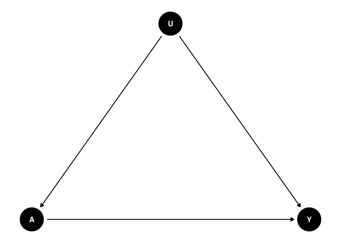
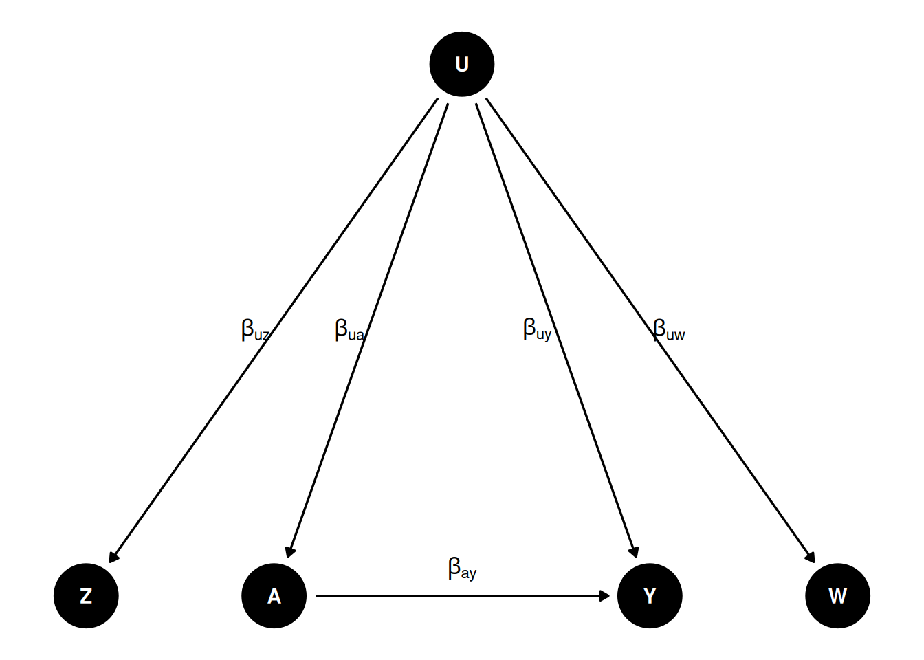
The central problem for observational studies is unobserved confounding. Even after conditioning on observed covariates \(X\), an unobserved confounder \(U\) may affect both treatment \(A\) and outcome \(Y\):
In this case, we have biased estimates of the treatment effect, regressing \(Y\) on \(A\) controlling for \(X\).
33.2 Proximal causal inference
Proximal causal inference (also called negative controls) is a framework that allows us to estimate the causal effect of treatment \(A\) on outcome \(Y\) while accounting for unobserved confounders.
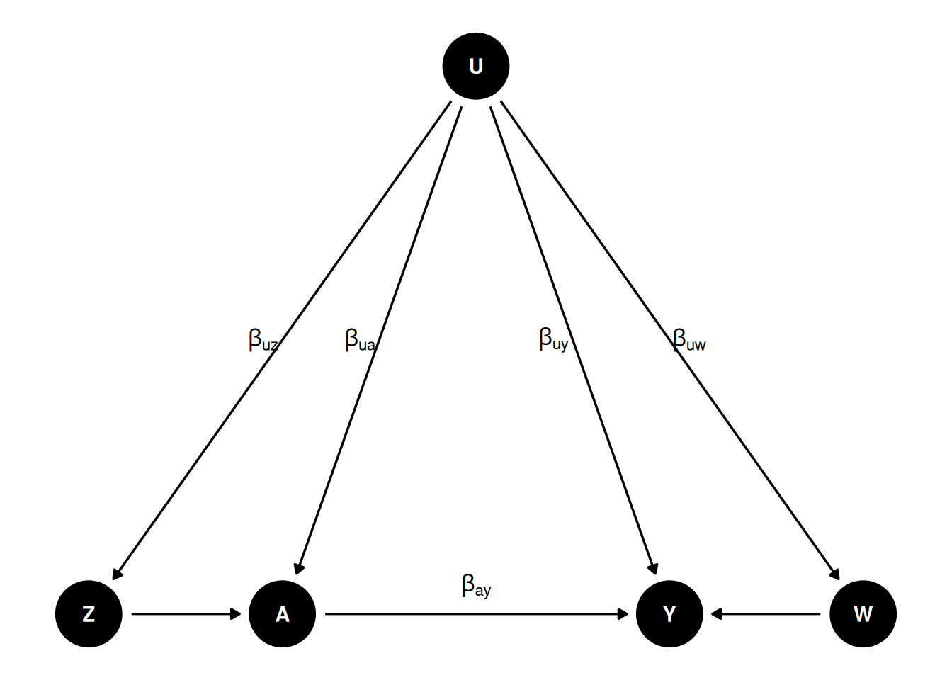
We’ll need a DAG like this:
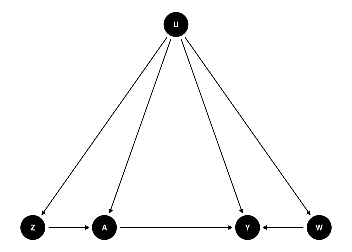
Basically we need two proxies for \(U\) to control for confounding. \(Z\) is called Negative Control for Exposure (NCE) and \(W\) is called Negative Control for Outcome (NCO). There is no link from \(Z\) to \(Y\), and no link from \(W\) to \(A\) or \(Z\).
\(Z\) is an NCE if \(Y(a,z) = Y(a)\) and \(Z \perp Y(a) | U\), meaning that \(Z\) satisfies the exclusion restriction that there is no direct link from \(Z\) to \(Y\), and that \(Z\) is independent of \(Y\) given \(U\).
\(W\) is an NCO if \(W(a,z) = W\) and \(W \perp (A,Z) | U\), meaning that \(A\) and \(Z\) have no direct link to \(W\).
33.2.1 Why this works
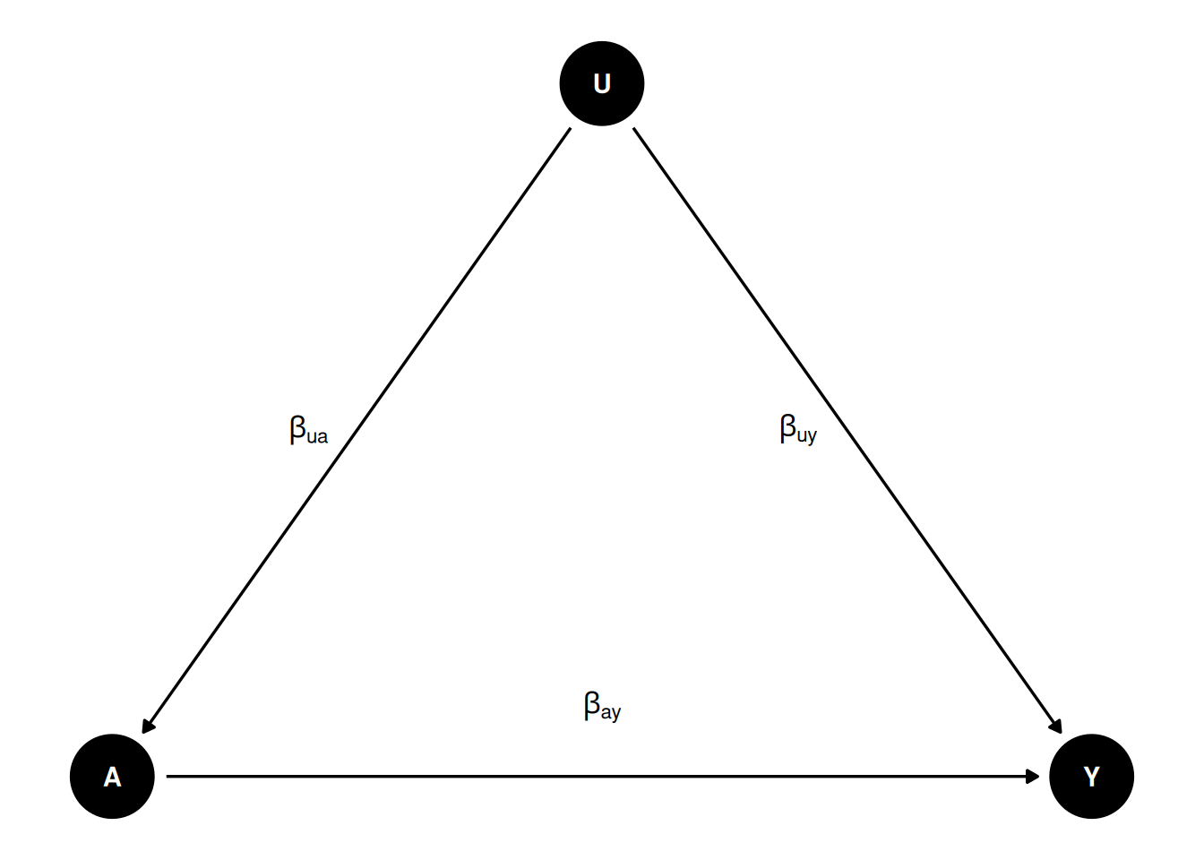
If we regress \(Y\) on \(A\), then we get \(\beta_{ay} + \beta_{uy} \beta_{ua}\), which is biased. How do we recover \(\beta_{ay}\)?
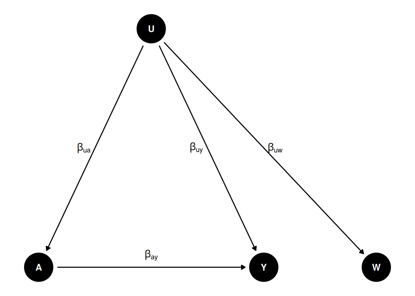
Suppose we have \(W\) as proxy of \(U\) and \(\beta_{uw} = \beta_{uy}\), then we can get the true effect. We can do regression of \(Y\) on \(A\), and then \(W\) on \(A\). The first regression gives us \(\beta_{ay} + \beta_{uy} \beta_{ua}\), and the second regression gives us \(\beta_{uw} \beta_{ua}\). We can then get \(\beta_{ay}\) from the difference of the two coefficients. This is similar to a DiD setting. Say \(W\) is \(Y_{t-1}\), and assume the effect of \(U\) is the same on \(Y\) and \(Y_{t-1}\), then effect of \(A\) on \(Y\) by the difference of regressing \(Y\) on \(A\) and \(Y_{t-1}\) on \(A\).
However, most likely \(\beta_{uw} \neq \beta_{uy}\). Then we need another proxy \(Z\) of \(U\) to recover the true effect. This is also called “double proxy”, or “double negative control”.
33.2.2 A linear model
Suppose we have the following linear model:
\[ E[Y | A,Z,U] = \beta_{y0} + \beta_{ay} A + \beta_{uy} U \tag{33.1}\] \[ E[W | A,Z,U] = \beta_{w0} + \beta_{uw} U \tag{33.2}\] \[ E[U | A,Z] = \beta_{u0} + \beta_{zu} Z + \beta_{au} A \tag{33.3}\]
\(\beta_{ay}\) is the true effect of \(A\) on \(Y\).
\[ E[Y | A,Z] = \beta_{y0} + \beta_{ay} A + \beta_{uy} (\beta_{u0} + \beta_{zu} Z + \beta_{au} A) \tag{33.4}\]
\[ E[W | A,Z] = \beta_{w0} + \beta_{uw} (\beta_{u0} + \beta_{zu} Z + \beta_{au} A) \tag{33.5}\]
From the last two regressions we can recover \(\beta_{ay}\):
If we define \(\delta_{a}^y = \beta_{ay} + \beta_{uy} \beta_{au}\) (regression coefficient of \(A\) on the \(Y\) regression) and \(\delta_{a}^w = \beta_{uw} \beta_{au}\), (regression coefficient of \(A\) on the \(W\) regression), similarly for \(\delta_z^y\) and \(\delta_z^w\), then we have
\[ \beta_{ay} = \delta_{a}^y - \delta_{a}^w \frac{\delta_z^y}{\delta_z^w} \tag{33.6}\]
In this linear-Gaussian special case only, we can look at this as a two-stage-least-squares-style regression and replace \(U\) with the predicted value of \(W\):
\[ E[Y | A,Z] = \left(\beta_{y0} - \frac{\beta_{uy}}{\beta_{uw}}\beta_{w0}\right) + \beta_{ay} A + \frac{\beta_{uy}}{\beta_{uw}} E[W | A,Z] \tag{33.7}\]
since \(E[U \mid A,Z] = (E[W \mid A,Z] - \beta_{w0})/\beta_{uw}\) from the \(W\) equation above. The coefficient on the predicted value of \(W\) is \(\beta_{uy}/\beta_{uw}\), not \(\beta_{uy}\) alone — it only reduces to \(\beta_{uy}\) when \(\beta_{uw}=1\). So we first regress \(W\) on \(A\) and \(Z\), then regress \(Y\) on \(A\) and the predicted value of \(W\).
This “predict \(W\) from \(A\) and \(Z\), then plug it in” shortcut is not the general proximal identification argument, and it is not the same as a standard IV/2SLS specification (we are not instrumenting an endogenous regressor with ivreg). In general proximal causal inference, the outcome bridge function \(h(A,W)\) is identified by solving the conditional moment restriction \(E[Y \mid A,Z] = E[h(A,W)\mid A,Z]\), which requires completeness (relevance) conditions linking the treatment-inducing proxy \(Z\) and the outcome-inducing proxy \(W\) to the hidden confounder \(U\). The generated regressor \(S = \widehat{E}[W\mid A,Z]\) is only a valid substitute under the linear-Gaussian structure above; even then the two-stage standard errors are wrong as written, because \(S\) is generated in the first stage (bootstrap the whole procedure).
33.2.3 A nonparametric model
We don’t have to have a linear model, this can be done with a nonparametric model as well.
\[ E[Y(a)] = E[h(a,W)] \tag{33.8}\] where \(E[Y | A,Z] = E[h(A,W) | A, Z]\).
That is, we can estimate \(h\) as a function of \(A\) and \(W\), identified using \(Z\), nonparametrically. This \(h\) function is called outcome bridge function. In the linear case, it is \(h(A, W) = \beta_0 + \beta_a A + \beta_w W\).
33.2.4 How to find proximal variables
Tchetgen Tchetgen and co-authors come up with a Data-driven Automated Negative Control Estimation (DANCE) algorithm to find negative controls. The idea is to use a machine learning algorithm to find the variables that are correlated with the treatment and the outcome, but not with the treatment and the outcome together. This is similar to the idea of finding instrumental variables.
33.3 example
Let’s generate data based on this DAG:
Code
set.seed(123)
n <- 5000
# Set coefficients
b_uw <- 0.5 # effect of U on W
b_uy <- 0.5 # effect of U on Y
b_ay <- 0.5 # effect of A on Y
b_uz <- 0.5 # effect of U on Z
b_ua <- 0.5 # effect of U on A
b_za <- 0.5 # effect of Z on A

U <- rnorm(n)
W <- b_uw * U + rnorm(n) # W is a function of U
Z <- b_uz * U + rnorm(n) # Z is a function of U
A <- b_ua * U + b_za * Z + rnorm(n) # A is a function of U and Z
Y <- b_uy * U + b_ay * A + rnorm(n) # Y is a function of U and A
# A <- rbinom(n, 1, plogis(-1 + U / 2)) # A is a binary treatment


# Create a data frame with the generated variables

data <- data.frame(W = W, Z = Z, A = A, Y = Y)
The simulation sets \(n = 5000\) and every coefficient to 0.5. The hidden confounder is \(U \sim N(0,1)\); the two proxies are \(W = 0.5U + \varepsilon_W\) and \(Z = 0.5U + \varepsilon_Z\); treatment is \(A = 0.5U + 0.5Z + \varepsilon_A\); and the outcome is \(Y = 0.5U + 0.5A + \varepsilon_Y\), all errors standard normal. The true effect of \(A\) on \(Y\) is therefore 0.5.
Note the roles: \(Z\) affects \(A\) but not \(Y\) directly, \(W\) is affected by \(U\) but affects nothing, and neither is a valid control for \(U\) on its own.
If we run regression of \(Y\) on \(A\), \(Z\), \(W\),
Call:
lm(formula = Y ~ A + Z + W, data = data)

Residuals:
    Min      1Q  Median      3Q     Max
-4.5836 -0.7167  0.0005  0.7305  4.4866

Coefficients:
             Estimate Std. Error t value Pr(>|t|)
(Intercept) -0.006347   0.015279  -0.415    0.678
A            0.660021   0.014123  46.734  < 2e-16 ***
Z            0.085004   0.016650   5.105 3.43e-07 ***
W            0.132798   0.014165   9.375  < 2e-16 ***
---
Signif. codes:  0 '***' 0.001 '**' 0.01 '*' 0.05 '.' 0.1 ' ' 1

Residual standard error: 1.08 on 4996 degrees of freedom
Multiple R-squared:  0.4556,    Adjusted R-squared:  0.4553
F-statistic:  1394 on 3 and 4996 DF,  p-value: < 2.2e-16
We don’t get the true effect of \(A\) on \(Y\): the coefficient on \(A\) is 0.660 against a true 0.5, a bias of 32%. Conditioning on both proxies does not remove the confounding, because neither \(W\) nor \(Z\) is \(U\) — each is a noisy reflection of it, and controlling for a noisy proxy leaves residual confounding. The proxies do carry signal (both are significant, at 0.085 and 0.133), which is what makes this failure mode deceptive: the regression looks like it is adjusting for the confounder.
If we do the 2sls using \(W\) and \(Z\), then we get the true effect.
Code
# Linear-Gaussian (Y, W) toy case ONLY. This two-stage plug-in identifies
# the effect under the linear structure above; it is not the general
# proximal estimator, and the reported SEs below are NOT valid because S is
# a generated regressor (bootstrap the whole two-step procedure for inference).
# Perform the first-stage linear regression W ~ A + Z
m1 <- lm(W ~ A + Z, data = data)
# Compute the estimated E[W|A,Z]
S <- m1$fitted.values
# Perform the second-stage linear regression Y ~ A + E[W|A,Z]
m2 <- lm(Y ~ A + S, data = data)
summary(m2)   # point estimate OK under the linear model; SEs need bootstrap
Call:
lm(formula = Y ~ A + S, data = data)

Residuals:
    Min      1Q  Median      3Q     Max
-4.5477 -0.7309  0.0059  0.7395  4.3715

Coefficients:
             Estimate Std. Error t value Pr(>|t|)
(Intercept) -0.005049   0.015408  -0.328    0.743
A            0.489342   0.043210  11.325  < 2e-16 ***
S            1.143480   0.199171   5.741 9.96e-09 ***
---
Signif. codes:  0 '***' 0.001 '**' 0.01 '*' 0.05 '.' 0.1 ' ' 1

Residual standard error: 1.089 on 4997 degrees of freedom
Multiple R-squared:  0.446, Adjusted R-squared:  0.4458
F-statistic:  2012 on 2 and 4997 DF,  p-value: < 2.2e-16
The two-stage estimate is 0.489, against the true 0.5 and the naive 0.660. Using the two proxies in the right way — one to build a predicted \(E[W \mid A, Z]\) and that prediction as the control — recovers the effect, where using both directly as regressors did not.
The reported standard error of 0.043 should be ignored, for the reason flagged in the code comment: \(S\) is a generated regressor, so the second-stage standard errors are wrong as written and need a bootstrap over both stages.