---
title: "Uplift Modeling and CATE"
author: "Xiang Ao"
date: "2025-10-10"
---
Uplift modeling is about estimating who changes because of treatment. In a
marketing example, this means separating people who buy because of the campaign
from people who would have bought anyway.
This is the same object as the conditional average treatment effect (CATE),
$$\tau(x) = E[Y(1) - Y(0) \mid X = x].$$ {#eq-uplift-1}
The word "uplift" is more common in industry. The word "CATE" is more common in
the causal inference literature.
## Python: causalml uplift trees
The `causalml` library (Uber) provides uplift tree classifiers and the
cumulative gain curve for evaluating targeting policies. The code below
follows the library's tutorial with synthetic data.
I am copying this code from <https://github.com/uber/causalml/blob/master/docs/examples/uplift_trees_with_synthetic_data.ipynb>.
> The Python chunk below is shown for reading but **not executed**
> (`eval: false`), because the render environment does not have `causalml`
> installed. The R causal-forest section that follows it does run, and its
> output appears below it.
```{python}
#| eval: false
import numpy as np
import pandas as pd

from causalml.dataset import make_uplift_classification
from causalml.inference.tree import UpliftRandomForestClassifier
from causalml.metrics import plot_gain

from sklearn.model_selection import train_test_split
import importlib
print(importlib.metadata.version('causalml') )

df, x_names = make_uplift_classification()
df.head()

# Look at the conversion rate and sample size in each group
df.pivot_table(values='conversion',
               index='treatment_group_key',
               aggfunc=[np.mean, np.size],
               margins=True)

# Split data to training and testing samples for model validation (next section)
df_train, df_test = train_test_split(df, test_size=0.2, random_state=111)

from causalml.inference.tree import UpliftTreeClassifier

clf = UpliftTreeClassifier(control_name='control')
clf.fit(df_train[x_names].values,
         treatment=df_train['treatment_group_key'].values,
         y=df_train['conversion'].values)
p = clf.predict(df_test[x_names].values)

df_res = pd.DataFrame(p, columns=clf.classes_)
df_res.head()

uplift_model = UpliftRandomForestClassifier(control_name='control')

uplift_model.fit(df_train[x_names].values,
                 treatment=df_train['treatment_group_key'].values,
                 y=df_train['conversion'].values)

df_res = uplift_model.predict(df_test[x_names].values, full_output=True)
print(df_res.shape)
df_res.head()

y_pred = uplift_model.predict(df_test[x_names].values)

# Put the predictions to a DataFrame for a neater presentation
# The output of `predict()` is a numpy array with the shape of [n_sample, n_treatment] excluding the
# predictions for the control group.
result = pd.DataFrame(y_pred,
                      columns=uplift_model.classes_[1:])
result.head()

# If all deltas are negative, assign to control; otherwise assign to the treatment
# with the highest delta
best_treatment = np.where((result < 0).all(axis=1),
                           'control',
                           result.idxmax(axis=1))

# Create indicator variables for whether a unit happened to have the
# recommended treatment or was in the control group
actual_is_best = np.where(df_test['treatment_group_key'] == best_treatment, 1, 0)
actual_is_control = np.where(df_test['treatment_group_key'] == 'control', 1, 0)

synthetic = (actual_is_best == 1) | (actual_is_control == 1)
synth = result[synthetic]

auuc_metrics = (synth.assign(is_treated = 1 - actual_is_control[synthetic],
                             conversion = df_test.loc[synthetic, 'conversion'].values,
                             uplift_tree = synth.max(axis=1))
                     .drop(columns=list(uplift_model.classes_[1:])))

plot_gain(auuc_metrics, outcome_col='conversion', treatment_col='is_treated')
```
A caution on this evaluation. The gain curve above keeps only the units whose
*observed* treatment happened to match the recommended treatment (or who were
controls), and then compares outcomes. This is a common tutorial shortcut, but
it estimates the value of the recommended policy **only if treatment was
randomly assigned** (so that "units who happened to get the recommended arm"
are exchangeable with those who did not). With observational treatment
assignment, this selection is itself confounded, and a valid off-policy
evaluation needs an inverse-probability / policy-value estimator that reweights
by the propensity of the observed treatment. Read the gain curve here as a
diagnostic under randomized assignment, not as a general off-policy evaluation.
## R: causal forest for CATE
In R, the `grf` package implements causal forests. The setup is simpler than
the uplift tree example: provide outcomes, treatments, and covariates, and the
forest estimates CATEs using honest splitting.
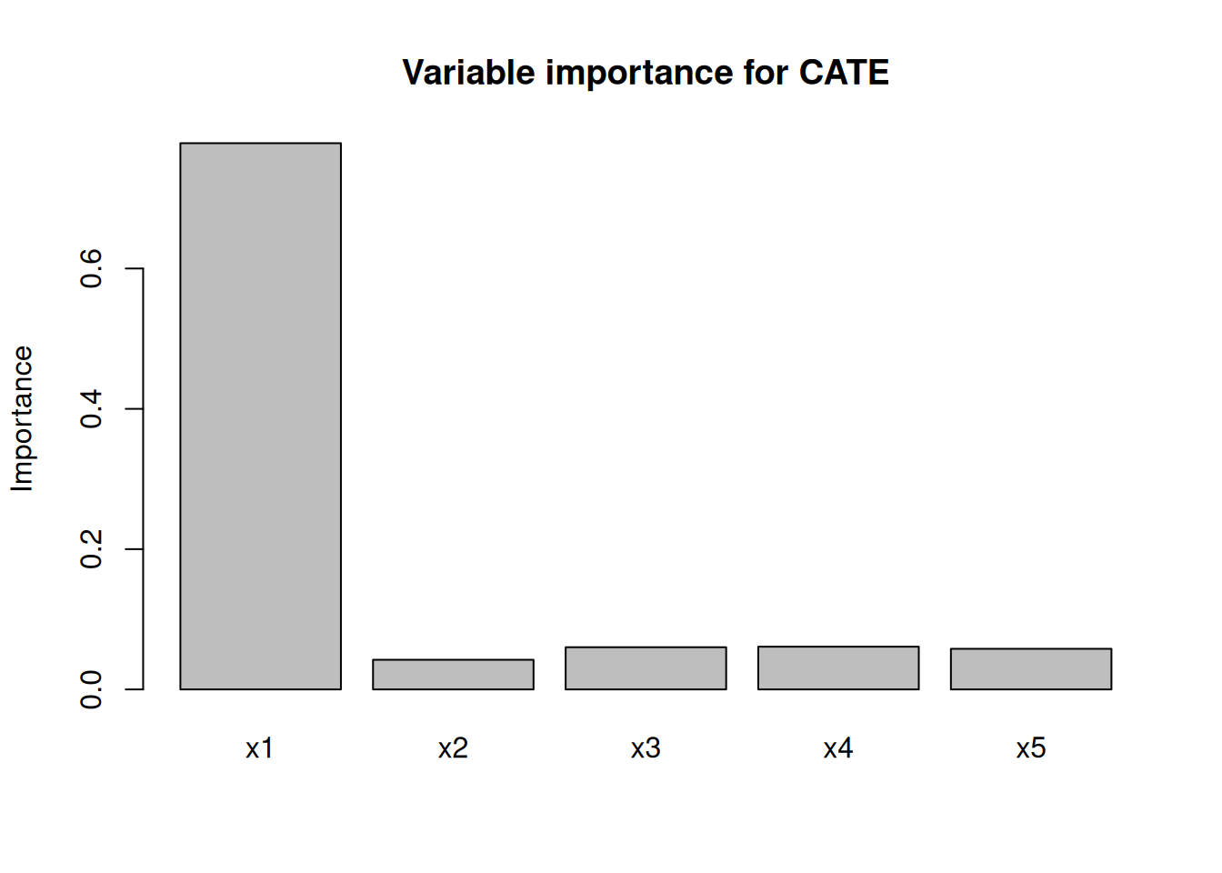
We simulate $n = 5000$ users with five independent standard normal covariates.
Treatment is randomly assigned, $W \sim \text{Bernoulli}(0.5)$, so there is no
confounding. The true CATE is $\tau(X) = 0.3 + 0.5X_1$ — the intervention helps
high-$x_1$ users more — and the outcome is
$Y = \tau(X)W + X_2 + \varepsilon$ with $\varepsilon \sim N(0, 0.5^2)$. The
average true effect is therefore 0.3, and only $x_1$ modifies it while $x_2$
affects the outcome level and $x_3$ to $x_5$ do nothing.
```{r}
#| echo: true
#| message: false
#| warning: false
#| cache: true
library(grf)
library(ggplot2)

# Simulate a marketing intervention
# True CATE: treatment helps high-engagement users more
set.seed(123)
n  <- 5000
X  <- matrix(rnorm(n * 5), n, 5)
colnames(X) <- paste0("x", 1:5)
W  <- rbinom(n, 1, 0.5)                          # random treatment
tau_true <- 0.3 + 0.5 * X[, 1]                   # CATE depends on x1
Y  <- tau_true * W + X[, 2] + rnorm(n, sd = 0.5) # observed outcome

# Fit causal forest
cf <- causal_forest(X, Y, W, num.trees = 2000, seed = 42)

# Estimate CATE for each unit
tau_hat <- predict(cf, estimate.variance = TRUE)
cate    <- tau_hat$predictions
cate_se <- sqrt(tau_hat$variance.estimates)

cat("Mean estimated CATE:", round(mean(cate), 3), "\n")
cat("True mean CATE: ", round(mean(tau_true), 3), "\n")
```
```{r}
#| echo: true
#| message: false
#| warning: false
#| cache: true
# Who benefits? Targeting policy
# Sort by predicted CATE, target top 30%
threshold <- quantile(cate, 0.70)
targeted  <- cate >= threshold

# Report the estimated and the simulated-true subgroup averages side by side.
# The first pair is what the forest predicts; the second is the truth under the
# same targeting rule, available here only because this is a simulation.
cat("Estimated CATE, targeted group:", round(mean(cate[targeted]), 3), "\n")
cat("Estimated CATE, non-targeted: ", round(mean(cate[!targeted]), 3), "\n")
cat("True CATE, targeted group:", round(mean(tau_true[targeted]), 3), "\n")
cat("True CATE, non-targeted: ", round(mean(tau_true[!targeted]), 3), "\n")
# Variable importance: which covariates drive heterogeneity?
# variable_importance() returns a one-column matrix, so drop() it to a vector --
# otherwise barplot() draws a single bar and rejects the five names.
imp <- drop(variable_importance(cf))
barplot(imp, names.arg = colnames(X),
        main = "Variable importance for CATE",
        ylab = "Importance")
```
```{r}
#| echo: true
#| message: false
#| warning: false
#| cache: true
# Omnibus test: is there significant CATE heterogeneity?
test_calibration(cf)
```
The forest gives a mean estimated CATE of 0.307 against the true 0.300. Sorting
on the estimate, the targeted group averages an *estimated* CATE of 0.858 against
0.071 for the rest. Because this is a simulation we can also look at the truth
under that same rule: 0.872 and 0.054, a roughly sixteenfold gap where the
estimates implied twelve. Either way the separation is wide, which is what makes
the targeting worth doing rather than treating everyone. The estimated pair is
what a practitioner would actually have; the true pair is available here only to
audit the exercise.
The `test_calibration()` output is a useful diagnostic. It checks whether units
with higher predicted CATEs also appear to have higher treatment effects.
## Uplift vs CATE: the same thing with different vocabulary
| Uplift term | Causal inference term |
|---|---|
| Uplift score | $\hat\tau(x)$ — estimated CATE |
| Persuadables | Covariate profiles with $\tau(x) > 0$ |
| Do-not-disturbs | Covariate profiles with $\tau(x) < 0$ |
| Cumulative gain curve | Policy value curve / AUTOC |
| Uplift tree | Causal tree / honest tree |
| Uplift forest | Causal forest (grf) |
The two vocabularies are not quite identical. "Persuadable" names an individual; $\tau(x)$ is an average over everyone sharing the profile $x$. A positive $\tau(x)$ says that subgroup gains on average. It does not say each member of it gains. Sorting individuals into persuadables and do-not-disturbs needs assumptions about individual potential outcomes, and a CATE does not supply them.
The Python `causalml` package comes from the marketing/tech vocabulary. `grf`
comes from the econometrics vocabulary. They are trying to estimate the same
quantity. For publication, I would usually want the inference and diagnostics
from `grf`. For a targeting exercise, the gain-curve tools in `causalml` are
also useful.
---
<!-- see-also-footer -->
*Systematic treatment: [R](https://xiangao.github.io/causal_econometrics_guide/heterogeneous-effects.html) · [Julia](https://xiangao.github.io/causal_econometrics_julia/heterogeneous-effects.html).*