I have a few posts about estimating ATE or CATE. The target has been getting the treatment effect or conditional treatment effect accurately. However, sometimes after estimating the treatment effects, we may be interested in the optimal treatment assignment. For example, a doctor may be interested in how to assign treatment based on patient characteristics. OSHA might be interested in which firms to send inspector to, based on firm characteristics, or past history. We may think we can just assign the treatment to those who benefited most (largest CATE), or any patient who has a positive CATE. However, the objective function for policy is different from the CATE target.
Suppose we have {Y(0), Y(1), X} and we have estimated the CATE as \(\tau(x)=E[Y(1)-Y(0)|X=x]\). The policy learning problem is to find a policy function that assigns treatment to maximize some utility function.
Suppose that policy is \[
\pi \ : \ X \rightarrow \{0,1\}
\tag{31.1}\] This policy is to assign treatment or control based on \(X\).
The natural objective function is a value function \(V(\pi) = E[Y_i(\pi(X_i))]\), which is the expected value of outcome with this policy. We’d like to maximize this function.
\[
V(\pi) = E[Y_i(\pi(X_i))] = E[Y_i(0)] + E[\tau(X) \pi(X)]
\tag{31.2}\] Since \(\pi\) only enters through \(E[\tau(X)\pi(X)]\), the maximizer is exactly \(\pi(X) = 1\{\tau(X) > 0\}\) — treat everyone with a positive effect. A threshold \(c \neq 0\) is not a free choice here: it appears once treatment is costly, where maximizing \(E[(\tau(X) - c)\pi(X)]\) gives the rule \(\tau(X) > c\) with \(c\) the per-unit cost. However, estimating \(\tau(X)\) is different from maximizing \(V\).
First, we don’t have the true \(\tau\). The loss function in estimating \(\tau(X)\) is different from the loss function in maximizing \(V\). The loss function in estimating \(\tau(X)\) is the squared error loss. We’ll see maximizing \(V\) is a different problem.
Second, the \(X\) we use to estimate \(\tau\) is different from the ones we can use for policy. For example, we have some variables used in CATE estimation that we cannot use for policy, like gender, or age, for discrimination reasons. Or there are variables we have after the experiment that we cannot use for CATE estimation, but we’d like to use for policy learning.
31.2 IPW loss
Kitagawa and Tetenov (2018) proposed a loss function for policy learning. The loss function is based on the inverse propensity weighting.
This is to say when we have \(W_i=\pi(X_i)\), we can use the outcome \(Y_i\) to estimate the value function. That is, when we have a policy, we then select the observations that matches that policy then weight the outcome by the inverse propensity score. This is to adjust the fact the there is selection bias for that policy. Therefore we re-weight it by IPW.
Obviously we don’t have the true propensity score of \(W_i=\pi(X_i)\), so we need to estimate it. We can estimate it by machine learning.
31.3 AIPW loss
The IPW loss can be not robust to model misspecification. Athey and Wager (2021) proposed a loss function that is robust to model misspecification. The loss function is based on the doubly robust estimator, AIPW.
Note the \(\Gamma_i\) is the score from the AIPW estimator. It’s basically the efficient influence function we learned from the nonparametric estimation of ATE.
One clarification about Equation 31.6, because the name is easy to over-read. With scalar doubly robust effect scores \(\hat\Gamma_i\), that quantity is a centered empirical welfare objective, not an estimate of the outcome-level policy value \(E[Y(\pi(X))]\). It has the same maximizer, up to an additive constant and a factor of two, which is all the optimization needs. An estimator of the value itself uses action-specific scores, or adds a control-outcome score to \(\pi(X_i)\hat\Gamma_i\). So maximize Equation 31.6, but do not report its value as the welfare of the learned rule.
We’d like to maximize this objective.
The basic idea is for each policy, calculate the score from AIPW estimator. Then calculate the value function. Then search over the policy space for the policy that maximizes the value function.
This is very computationally intensive task. Right now seems it would work for “shallow” trees. That is, we allow 2 or 3 levels of trees. Otherwise, the search space could be too large to search.
31.4 Policytree
The simulation is built so that the optimal policy is known. We draw \(n = 1000\) observations with ten independent standard normal covariates. The propensity is \(e(X) = 1/(1+e^{X_3})\), so treatment depends on \(X_3\) alone. The true CATE is
and the outcome is \(Y = X_3 + W\tau(X) + N(0,1)\).
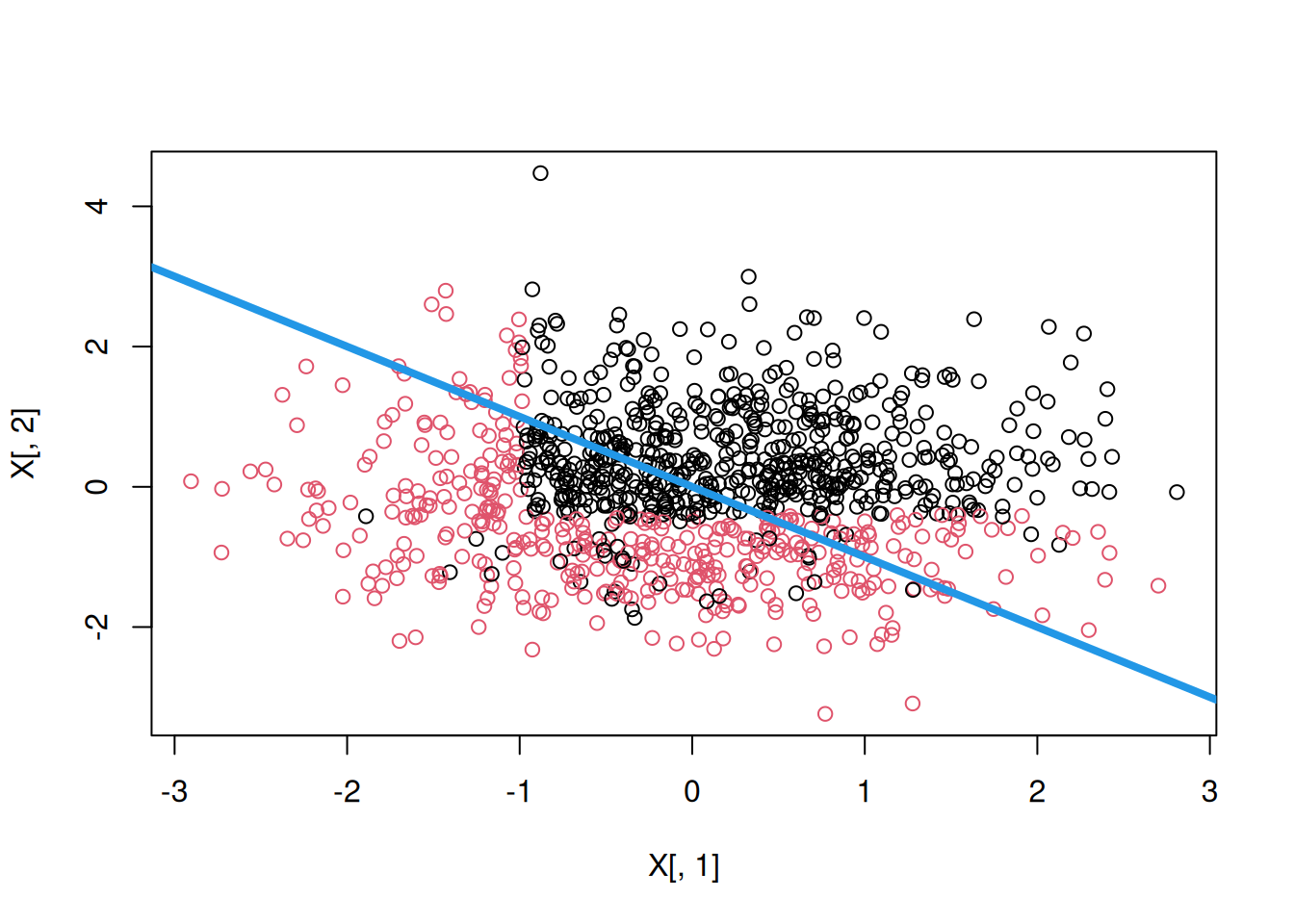
Because \(\tau(X) > 0\) exactly when \(X_1 + X_2 < 0\), the optimal policy is the half-plane below the line \(X_1 + X_2 = 0\) — which is the diagonal drawn on the last plot. Note that only \(X_1\) and \(X_2\) matter for the policy, \(X_3\) matters only for selection, and \(X_4\) through \(X_{10}\) are pure noise.
plot(X[, 1], X[, 2], col =pp)abline(0, -1, lwd =4, col =4)
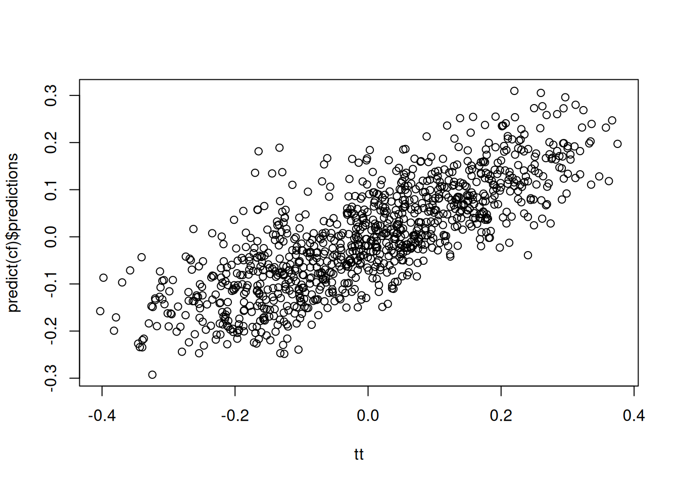
In the example, first “causal_forest” is used to estimate the CATE. “double_robust_scores” is used to calculate the AIPW score. Then “policy_tree” is used to estimate the policy tree. The level of tree is set to 2.
Read the fitted tree against the truth rather than on its own terms. The optimal rule is a diagonal boundary, \(X_1 + X_2 < 0\), and a depth-2 axis-aligned tree cannot represent a diagonal at all — the best it can do is approximate it with at most three perpendicular cuts. The tree therefore splits on whichever variables happen to reduce the loss most, and because the true signal is spread across a diagonal it may not select \(X_1\) or \(X_2\) at all — runs of this chunk routinely split entirely on noise covariates such as \(X_8\) and \(X_{10}\). That is worth seeing rather than explaining away: when the policy class cannot express the optimal rule, the fitted splits carry little information about which variables matter. The last plot makes this visible: the coloured regions are rectangles, the true boundary is the drawn line, and the mismatch between them is the approximation error of the policy class, not an estimation failure.
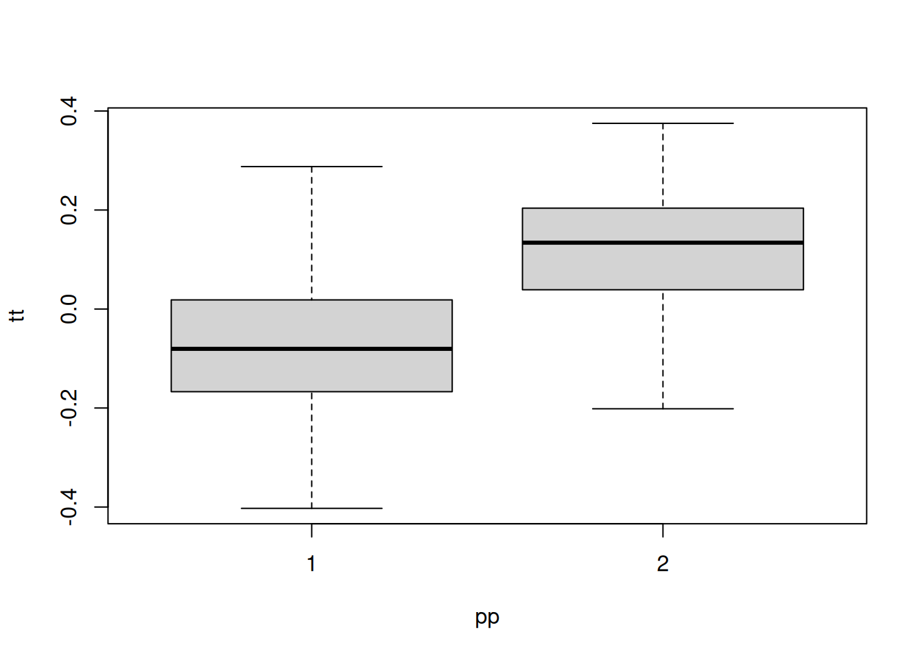
The boxplot(tt ~ pp) is the honest summary: it shows the distribution of the true effect within each recommended action. A good rule puts most of the positive-\(\tau\) mass in the “treat” box.
Note that this chunk sets no seed, so the covariates, the forest and therefore the fitted splits differ on every execution. The qualitative reading above is stable; the particular variables and cut points printed are not.
---title: "Policy learning by policytree"date: "2024-03-22"---## Optimal policyI have a few posts about estimating ATE or CATE. The target has been getting the treatment effect or conditional treatment effect accurately. However, sometimes after estimating the treatment effects, we may be interested in the optimal treatment assignment. For example, a doctor may be interested in how to assign treatment based on patient characteristics. OSHA might be interested in which firms to send inspector to, based on firm characteristics, or past history. We may think we can just assign the treatment to those who benefited most (largest CATE), or any patient who has a positive CATE. However, the objective function for policy is different from the CATE target.Suppose we have {Y(0), Y(1), X} and we have estimated the CATE as $\tau(x)=E[Y(1)-Y(0)|X=x]$. The policy learning problem is to find a policy function that assigns treatment to maximize some utility function.Suppose that policy is$$\pi \ : \ X \rightarrow \{0,1\}$$ {#eq-policytree-1}This policy is to assign treatment or control based on $X$.The natural objective function is a value function $V(\pi) = E[Y_i(\pi(X_i))]$, which is the expected value of outcome with this policy. We'd like to maximize this function.$$V(\pi) = E[Y_i(\pi(X_i))] = E[Y_i(0)] + E[\tau(X) \pi(X)]$$ {#eq-policytree-2}Since $\pi$ only enters through $E[\tau(X)\pi(X)]$, the maximizer is exactly$\pi(X) = 1\{\tau(X) > 0\}$ --- treat everyone with a positive effect. Athreshold $c \neq 0$ is not a free choice here: it appears once treatment iscostly, where maximizing $E[(\tau(X) - c)\pi(X)]$ gives the rule$\tau(X) > c$ with $c$ the per-unit cost. However, estimating $\tau(X)$ is different from maximizing $V$.First, we don't have the true $\tau$. The loss function in estimating $\tau(X)$ is different from the loss function in maximizing $V$. The loss function in estimating $\tau(X)$ is the squared error loss. We'll see maximizing $V$ is a different problem.Second, the $X$ we use to estimate $\tau$ is different from the ones we can use for policy. For example, we have some variables used in CATE estimation that we cannot use for policy, like gender, or age, for discrimination reasons. Or there are variables we have after the experiment that we cannot use for CATE estimation, but we'd like to use for policy learning.## IPW lossKitagawa and Tetenov (2018) proposed a loss function for policy learning. The loss function is based on the inverse propensity weighting.$$\hat \pi = argmax \{ \hat V(\pi) : \pi \in \Pi \}$$ {#eq-policytree-3}$$ \hat V(\pi) = \frac{1}{n} \sum_{i=1}^n \frac{1({W_i=\pi(X_i)})} {P[W_i=\pi(X_i) | X_i]} Y_i$$ {#eq-policytree-4}This is to say when we have $W_i=\pi(X_i)$, we can use the outcome $Y_i$ to estimate the value function. That is, when we have a policy, we then select the observations that matches that policy then weight the outcome by the inverse propensity score. This is to adjust the fact the there is selection bias for that policy. Therefore we re-weight it by IPW.Obviously we don't have the true propensity score of $W_i=\pi(X_i)$, so we need to estimate it. We can estimate it by machine learning.## AIPW lossThe IPW loss can be not robust to model misspecification. Athey and Wager (2021) proposed a loss function that is robust to model misspecification. The loss function is based on the doubly robust estimator, AIPW.$$\hat \pi = argmax \{ \hat V(\pi) : \pi \in \Pi \}$$ {#eq-policytree-5}$$ \hat V(\pi) = \frac{1}{n} \sum_{i=1}^n (2\pi(X_i)-1) \hat \Gamma_i$$ {#eq-policytree-6}$$ \Gamma_i = \hat \mu(1)(X_i) - \hat \mu(0)(X_i) + \frac{W_i}{\hat e(X_i)}(Y_i - \hat \mu(1) (X_i)) - \frac{1-W_i}{1-\hat e(X_i)}(Y_i - \hat \mu(0) (X_i))$$ {#eq-policytree-7}Note the $\Gamma_i$ is the score from the AIPW estimator. It's basically the efficient influence function we learned from the nonparametric estimation of ATE.One clarification about @eq-policytree-6, because the name is easy to over-read. With scalar doubly robust effect scores $\hat\Gamma_i$, that quantity is a *centered empirical welfare objective*, not an estimate of the outcome-level policy value $E[Y(\pi(X))]$. It has the same maximizer, up to an additive constant and a factor of two, which is all the optimization needs. An estimator of the value itself uses action-specific scores, or adds a control-outcome score to $\pi(X_i)\hat\Gamma_i$. So maximize @eq-policytree-6, but do not report its value as the welfare of the learned rule.We'd like to maximize this objective.The basic idea is for each policy, calculate the score from AIPW estimator. Then calculate the value function. Then search over the policy space for the policy that maximizes the value function.This is very computationally intensive task. Right now seems it would work for "shallow" trees. That is, we allow 2 or 3 levels of trees. Otherwise, the search space could be too large to search.## PolicytreeThe simulation is built so that the optimal policy is known. We draw $n = 1000$observations with ten independent standard normal covariates. The propensity is$e(X) = 1/(1+e^{X_3})$, so treatment depends on $X_3$ alone. The true CATE is$$\tau(X) = \frac{1}{1 + e^{(X_1+X_2)/2}} - \tfrac12,$$ {#eq-policytree-8}and the outcome is $Y = X_3 + W\tau(X) + N(0,1)$.Because $\tau(X) > 0$ exactly when $X_1 + X_2 < 0$, the optimal policy is thehalf-plane below the line $X_1 + X_2 = 0$ — which is the diagonal drawn on thelast plot. Note that only $X_1$ and $X_2$ matter for the policy, $X_3$ mattersonly for selection, and $X_4$ through $X_{10}$ are pure noise.```{r}#| echo: true#| message: falselibrary(grf)library(policytree)library(DiagrammeR)n <-1000p <-10X <-matrix(rnorm(n * p), n, p)ee <-1/ (1+exp(X[, 3]))tt <-1/ (1+exp((X[, 1] + X[, 2]) /2)) -0.5W <-rbinom(n, 1, ee)Y <- X[, 3] + W * tt +rnorm(n)cf <-causal_forest(X, Y, W)plot(tt, predict(cf)$predictions)dr <-double_robust_scores(cf)tree <-policy_tree(X, dr, 2)treepp <-predict(tree, X)boxplot(tt ~ pp)plot(tree)plot(X[, 1], X[, 2], col = pp)abline(0, -1, lwd =4, col =4)```In the example, first "causal_forest" is used to estimate the CATE. "double_robust_scores" is used to calculate the AIPW score. Then "policy_tree" is used to estimate the policy tree. The level of tree is set to 2.Read the fitted tree against the truth rather than on its own terms. The optimalrule is a *diagonal* boundary, $X_1 + X_2 < 0$, and a depth-2 axis-aligned treecannot represent a diagonal at all — the best it can do is approximate it withat most three perpendicular cuts. The tree therefore splits on whichever variables happen to reduce the loss most,and because the true signal is spread across a diagonal it may not select $X_1$or $X_2$ at all — runs of this chunk routinely split entirely on noisecovariates such as $X_8$ and $X_{10}$. That is worth seeing rather thanexplaining away: when the policy class cannot express the optimal rule, thefitted splits carry little information about which variables matter. The last plot makes this visible: the coloured regions arerectangles, the true boundary is the drawn line, and the mismatch between themis the approximation error of the policy class, not an estimation failure.The `boxplot(tt ~ pp)` is the honest summary: it shows the distribution of the*true* effect within each recommended action. A good rule puts most of thepositive-$\tau$ mass in the "treat" box.Note that this chunk sets no seed, so the covariates, the forest and thereforethe fitted splits differ on every execution. The qualitative reading above isstable; the particular variables and cut points printed are not.---<!-- see-also-footer -->*Systematic treatment: [R](https://xiangao.github.io/causal_econometrics_guide/heterogeneous-effects.html) · [Julia](https://xiangao.github.io/causal_econometrics_julia/heterogeneous-effects.html).*