11 Bayesian Causal Inference
The earlier chapters mostly compute point estimates and standard errors. Bayesian methods instead put priors on unknown quantities and return a posterior distribution. For causal inference this is useful when we want uncertainty about a function of the model, such as an individual treatment effect or a policy value, not just one coefficient.
I use two models:
- BART for causal inference (Hill 2011), where BART is used as a flexible outcome model.
- Bayesian Causal Forests (BCF; Hahn, Murray, & Carvalho 2020), which separates the baseline outcome model from the treatment-effect model.
Related reading: The chapter Using Numpyro in Topics on Econometrics and Causal Inference demonstrates a Bayesian hierarchical model with Numpyro. For an MCMC-from-scratch perspective on causal inference, that companion piece is the natural next step after this chapter.
11.1 Setup
I use the same simulation as in the Heterogeneous Treatment Effects chapter. The true treatment effect varies with X1.
set.seed(42)
n <- 2000
p <- 5

X <- matrix(runif(n * p), n, p)
colnames(X) <- paste0("X", 1:p)
# Treatment depends only on observed covariates, so unconfoundedness given X
# holds and the "True ATE" comparison measures estimator performance (not bias).
ps <- plogis(-0.3 + 1.5 * X[, 2])
D  <- rbinom(n, 1, ps)
tau <- 1 + 2 * X[, 1]
Y0  <- 0.5 * X[, 2] + rnorm(n)
Y1  <- Y0 + tau
Y   <- ifelse(D == 1, Y1, Y0)

df <- data.frame(Y = Y, D = D, X)
cat(sprintf("True ATE = %.3f\n", mean(tau)))
True ATE = 1.98511.2 BART for causal inference (Hill 2011)
BART is a sum of many small regression trees. The prior keeps each tree weak, and the sum of trees gives flexibility.
For causal inference, the recipe is:
- Fit BART for \(\mu(d,x)=\mathbb{E}[Y \mid D=d,X=x]\).
- For each unit \(i\), predict counterfactuals \(\mu(1, x_i)\) and \(\mu(0, x_i)\).
- The individual treatment effect (ITE) is \(\hat\tau_i = \mu(1, x_i) - \mu(0, x_i)\).
- Average the posterior draws to get the posterior for ATE or ITEs.
*****Into main of wbart
*****Data:
data:n,p,np: 2000, 6, 0
y1,yn: 2.058453, -2.423620
x1,x[n*p]: 1.000000, 0.647277
*****Number of Trees: 200
*****Number of Cut Points: 1 ... 100
*****burn and ndpost: 200, 1000
*****Prior:beta,alpha,tau,nu,lambda: 2.000000,0.950000,0.174777,3.000000,0.205658
*****sigma: 1.027514
*****w (weights): 1.000000 ... 1.000000
*****Dirichlet:sparse,theta,omega,a,b,rho,augment: 0,0,1,0.5,1,6,0
*****nkeeptrain,nkeeptest,nkeeptestme,nkeeptreedraws: 1000,1000,1000,1000
*****printevery: 1000
*****skiptr,skipte,skipteme,skiptreedraws: 1,1,1,1

MCMC
done 0 (out of 1200)
done 1000 (out of 1200)
time: 15s
check counts
trcnt,tecnt,temecnt,treedrawscnt: 1000,0,0,1000*****In main of C++ for bart prediction
tc (threadcount): 1
number of bart draws: 1000
number of trees in bart sum: 200
number of x columns: 6
from x,np,p: 6, 2000
***using serial codemu0_post <- predict(bart_fit, newdata = X_control)*****In main of C++ for bart prediction
tc (threadcount): 1
number of bart draws: 1000
number of trees in bart sum: 200
number of x columns: 6
from x,np,p: 6, 2000
***using serial code# Posterior of individual treatment effects
tau_post <- mu1_post - mu0_post # 1000 x n posterior draws of ITEs
# Posterior summaries
tau_mean <- rowMeans(tau_post) # ATE in each draw
ate_post_mean <- mean(tau_mean)
ate_post_sd <- sd(tau_mean)
ate_post_ci <- quantile(tau_mean, c(0.025, 0.975))
cat(sprintf("BART ATE posterior:\n"))BART ATE posterior: Mean: 1.977 SD: 0.048 95% CrI: [1.880, 2.071] True ATE: 1.985The posterior draws give the uncertainty in the ATE directly.
11.2.1 Individual-level credible intervals
BART also gives a posterior for each unit’s treatment effect. Here I plot the posterior mean and pointwise credible intervals against the true \(\tau_i\).
ite_mean <- colMeans(tau_post)
ite_lo   <- apply(tau_post, 2, quantile, 0.025)
ite_hi   <- apply(tau_post, 2, quantile, 0.975)

df_ite <- tibble(
  X1     = X[, 1],
  true   = tau,
  est    = ite_mean,
  lo     = ite_lo,
  hi     = ite_hi
)

ggplot(df_ite, aes(x = X1)) +
  geom_ribbon(aes(ymin = lo, ymax = hi), alpha = 0.2,
              fill = "steelblue") +
  geom_point(aes(y = est), size = 0.4, alpha = 0.3, colour = "steelblue") +
  geom_abline(aes(intercept = 1, slope = 2), colour = "firebrick",
              linetype = "dashed", linewidth = 1) +
  labs(x = "X1", y = "Individual treatment effect",
       caption = "Red dashed = true τ(x). Blue band = pointwise 95% credible interval.") +
  theme_minimal()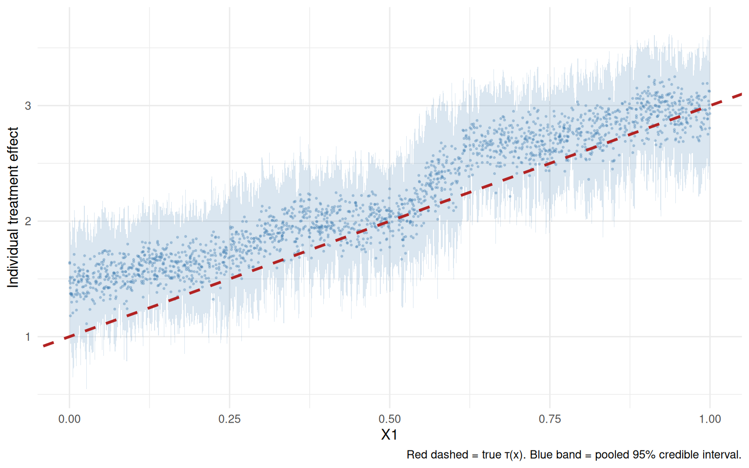
The blue ribbon is the pointwise 95% credible interval. The red dashed line is the true treatment-effect function.
11.3 Bayesian Causal Forests (BCF)
BART models \(\mathbb{E}[Y \mid D,X]\) directly. That means the same trees have to learn the baseline outcome and the treatment-effect heterogeneity. When strong predictors of \(Y(0)\) are also related to treatment, this can create noisy treatment-effect estimates.
BCF writes the conditional mean as
\[ \mathbb{E}[Y \mid D, X] = \mu(X) + \tau(X)\, D, \]
and puts separate priors on \(\mu(X)\) and \(\tau(X)\). The treatment-effect part is regularized more strongly, which helps avoid overfitting heterogeneity.
# BCF requires a propensity score as an input ("piHat")
ps_fit <- glm(D ~ X1 + X2 + X3 + X4 + X5, data = df, family = binomial)
piHat  <- predict(ps_fit, type = "response")

# BCF prints MCMC progress in a way that conflicts with knitr's encoding.
# Its `verbose=FALSE`/`no_output=TRUE` arguments do not fully suppress this
# within the SAME R session (the progress output comes from C++ code, not
# from R's own message()/cat() machinery that sink()/suppressMessages()
# can intercept) -- so the only reliable fix is running bcf() in its own R
# process and only reading back the saved result, never its console output.
# Use SEPARATE input and output files so a failed subprocess can never leave
# the input list sitting where we expect the result, and check the exit
# status and object names before trusting it.
tmp_in  <- tempfile(fileext = ".rds")
tmp_out <- tempfile(fileext = ".rds")
tmp_err <- tempfile(fileext = ".log")
saveRDS(list(Y = df$Y, D = df$D, X = X, piHat = piHat), tmp_in)
status <- system(paste0("Rscript -e '",
  "args <- readRDS(\"", tmp_in, "\"); ",
  "suppressMessages(library(bcf)); ",
  "f <- bcf(y=args$Y, z=args$D, x_control=args$X, x_moderate=args$X, ",
  "pihat=args$piHat, nburn=200, nsim=1000, n_chains=1, no_output=TRUE, ",
  "verbose=FALSE); ",
  "saveRDS(list(tau=f$tau), \"", tmp_out, "\")'"),
  ignore.stdout = TRUE, ignore.stderr = FALSE)
# Surface the real cause instead of failing far downstream on a missing field.
if (status != 0L || !file.exists(tmp_out)) {
  stop("BCF subprocess failed (exit status ", status, "). ",
       "Check that the 'bcf' package is installed in the worker session.")
}
bcf_fit <- readRDS(tmp_out)
if (is.null(bcf_fit$tau)) {
  stop("BCF subprocess produced no 'tau' draws; aborting.")
}
unlink(c(tmp_in, tmp_out, tmp_err))
Now extract the posterior treatment effects:
BCF ATE posterior: Mean: 1.982 SD: 0.046 95% CrI: [1.897, 2.072] True ATE: 1.98511.3.1 BART vs BCF: individual treatment effects
Compare the estimated CATEs:
df_compare <- bind_rows(
  tibble(X1 = X[, 1], est = bcf_ite_mean, true = tau, method = "BCF"),
  tibble(X1 = X[, 1], est = ite_mean,     true = tau, method = "BART")
)

ggplot(df_compare, aes(X1, est)) +
  geom_point(alpha = 0.2, size = 0.3, colour = "steelblue") +
  geom_smooth(method = "loess", se = FALSE, colour = "darkblue",
              linewidth = 1) +
  geom_abline(intercept = 1, slope = 2, linetype = "dashed",
              colour = "firebrick") +
  facet_wrap(~ method) +
  labs(x = "X1", y = "Estimated ITE",
       caption = "Red dashed = truth = 1 + 2 X1") +
  theme_minimal()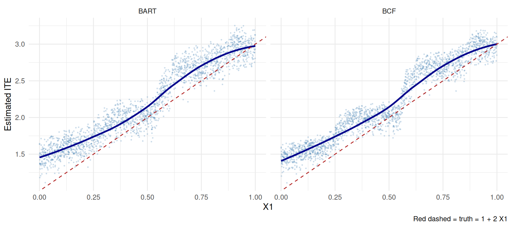
BCF is usually smoother because it separates the prognostic and treatment effect parts of the model.
11.4 When to use Bayesian methods
| Reason to use Bayesian | Reason to use Frequentist |
|---|---|
| Prior information matters | Asymptotic theory is well-understood |
| Need full posterior (e.g. for downstream decisions) | Computational cost matters (BART is slow on large \(n\)) |
| Hierarchical / multilevel data structure | Effects are simple averages |
| Small sample, weak identification | Effects are well-identified |
| Want individual-level CrIs | Existing frequentist toolkit is sufficient |
Bayesian methods are most useful when the posterior itself will be used: for individual treatment decisions, policy values, or hierarchical models. If the target is just a well-identified ATE in a large sample, the frequentist methods in earlier chapters are often simpler.
11.5 Practical guidance
- Start with BCF if the goal is heterogeneous effects.
- Check MCMC diagnostics. A bad chain makes the posterior summaries useless.
- For BCF, pay attention to
piHat; it is part of the model input. - Report posterior mean, posterior SD, and credible intervals for ATE and meaningful CATE summaries.
11.6 Connections
- The Heterogeneous Treatment Effects chapter covers frequentist meta-learners (S/T/X/R/DR) and causal forests via
grf. BCF can be viewed as the Bayesian counterpart to causal forests: both use ensembles of trees, but BCF puts priors on the trees whilegrfuses honest sample-splitting. - The Sensitivity Analysis chapter’s Cinelli-Hazlett bounds are frequentist; the Bayesian analog is a prior on the unmeasured-confounder strength (cf. McCandless et al. 2007).
- For Bayesian Numpyro-style hierarchical models, see the companion blog chapter.
11.7 Summary
- BART estimates counterfactual outcomes by fitting a flexible outcome model.
- BCF separates baseline outcome prediction from treatment-effect heterogeneity.
- The main output is the posterior, especially for individual effects or policy decisions.
- Computation is the main cost. For very large data, frequentist HTE methods are usually easier.