7 Matching Estimators
Matching is a way to make treated and control observations more comparable. For each treated observation, we look for controls with similar covariates. Then we compare outcomes in this matched sample.
This does not solve endogeneity. Matching only helps with selection on observables. If the treatment is selected on unobserved variables, matching will not fix the problem. The value of matching is that it makes the overlap problem visible. A regression can extrapolate quietly; matching often shows that there are no good controls for part of the treated sample.
In R, the main workflow is MatchIt for matching and cobalt for balance checking.
Related reading: A longer treatment is in Matching and Weighting Part 1 of Topics on Econometrics and Causal Inference, which credits Noah Greifer and coauthors (the
MatchIt/WeightItpackage authors).
7.1 Assumptions
Matching needs the same assumptions as other selection-on-observables methods:
- SUTVA — no interference, no hidden treatment versions.
- Ignorability (unconfoundedness) — conditional on \(X\), the treatment \(D\) is independent of the potential outcomes \((Y(0), Y(1))\).
- Overlap (positivity) — every value of \(X\) has positive probability of being both treated and untreated.
Even if ignorability is true, the covariate distribution can be very different in the treated and control groups. Matching tries to repair that before estimating the effect. If there is no overlap, it should not pretend there is overlap.
7.2 The Lalonde example
I use the Lalonde job-training data because it is the standard example for matching. The treatment is job training. The outcome is 1978 earnings. The data set in MatchIt is the observational version, so the treated and control groups are not balanced at the start.
Rows: 614
Columns: 9
$ treat    <int> 1, 1, 1, 1, 1, 1, 1, 1, 1, 1, 1, 1, 1, 1, 1, 1, 1, 1, 1, 1, 1…
$ age      <int> 37, 22, 30, 27, 33, 22, 23, 32, 22, 33, 19, 21, 18, 27, 17, 1…
$ educ     <int> 11, 9, 12, 11, 8, 9, 12, 11, 16, 12, 9, 13, 8, 10, 7, 10, 13,…
$ race     <fct> black, hispan, black, black, black, black, black, black, blac…
$ married  <int> 1, 0, 0, 0, 0, 0, 0, 0, 0, 1, 0, 0, 0, 1, 0, 0, 0, 0, 0, 0, 0…
$ nodegree <int> 1, 1, 0, 1, 1, 1, 0, 1, 0, 0, 1, 0, 1, 1, 1, 1, 0, 1, 0, 0, 1…
$ re74     <dbl> 0, 0, 0, 0, 0, 0, 0, 0, 0, 0, 0, 0, 0, 0, 0, 0, 0, 0, 0, 0, 0…
$ re75     <dbl> 0, 0, 0, 0, 0, 0, 0, 0, 0, 0, 0, 0, 0, 0, 0, 0, 0, 0, 0, 0, 0…
$ re78     <dbl> 9930.0460, 3595.8940, 24909.4500, 7506.1460, 289.7899, 4056.4…
The treatment is treat; the outcome is re78; the covariates are age, educ, race, married, nodegree, re74, and re75.
First check balance before doing any matching:
Balance Measures
                Type Diff.Un     M.Threshold.Un
distance    Distance  1.7941
age          Contin. -0.3094 Not Balanced, >0.1
educ         Contin.  0.0550     Balanced, <0.1
race_black    Binary  0.6404 Not Balanced, >0.1
race_hispan   Binary -0.0827     Balanced, <0.1
race_white    Binary -0.5577 Not Balanced, >0.1
married       Binary -0.3236 Not Balanced, >0.1
nodegree      Binary  0.1114 Not Balanced, >0.1
re74         Contin. -0.7211 Not Balanced, >0.1
re75         Contin. -0.2903 Not Balanced, >0.1

Balance tally for mean differences
                   count
Balanced, <0.1         2
Not Balanced, >0.1     7

Variable with the greatest mean difference
 Variable Diff.Un     M.Threshold.Un
     re74 -0.7211 Not Balanced, >0.1

Sample sizes
    Control Treated
All     429     185
Several standardized mean differences are larger than 0.1. That is usually too large to call the sample balanced.
7.3 Distance measures
Matching needs a distance metric. The usual choices are:
- Propensity score: estimate \(\hat e(x)=P(D=1 \mid X=x)\) and match on the fitted probability. This turns many covariates into one score.
- Mahalanobis distance: match on the raw covariates using the squared distance \((x_i-x_j)'\Sigma^{-1}(x_i-x_j)\) (rankings are unchanged by the square root). This works better in low dimension.
- Hybrid: impose a propensity-score caliper, then use Mahalanobis distance inside the caliper.
7.4 Matching methods
7.4.1 Nearest-neighbour matching on a propensity score
m.nn <- matchit(treat ~ age + educ + race + married + nodegree + re74 + re75,
                data = lalonde,
                method = "nearest",
                distance = "glm",
                link = "linear.logit",
                ratio = 1)

m.nn
A `matchit` object
- method: 1:1 nearest neighbor matching without replacement
- distance: Propensity score
- estimated with logistic regression and linearized
- number of obs.: 614 (original), 370 (matched)
- target estimand: ATT
- covariates: age, educ, race, married, nodegree, re74, re75Now check balance again:
Balance Measures
                Type Diff.Adj        M.Threshold
distance    Distance   0.9192
age          Contin.   0.0718     Balanced, <0.1
educ         Contin.  -0.1290 Not Balanced, >0.1
race_black    Binary   0.3730 Not Balanced, >0.1
race_hispan   Binary  -0.1568 Not Balanced, >0.1
race_white    Binary  -0.2162 Not Balanced, >0.1
married       Binary  -0.0216     Balanced, <0.1
nodegree      Binary   0.0703     Balanced, <0.1
re74         Contin.  -0.0505     Balanced, <0.1
re75         Contin.  -0.0257     Balanced, <0.1

Balance tally for mean differences
                   count
Balanced, <0.1         5
Not Balanced, >0.1     4

Variable with the greatest mean difference
   Variable Diff.Adj        M.Threshold
 race_black    0.373 Not Balanced, >0.1

Sample sizes
          Control Treated
All           429     185
Matched       185     185
Unmatched     244       0
Some covariates are still not balanced. Nearest-neighbor matching on a logit propensity score is simple, but it is not automatically good.
7.4.2 Full matching
Full matching forms subclasses with treated and control observations inside each subclass. It can put one treated unit with several controls, or one control with several treated units. It uses all observations and then assigns weights.
Balance Measures
                Type Diff.Adj    M.Threshold
distance    Distance   0.0045 Balanced, <0.1
age          Contin.   0.0393 Balanced, <0.1
educ         Contin.  -0.0956 Balanced, <0.1
race_black    Binary   0.0043 Balanced, <0.1
race_hispan   Binary   0.0103 Balanced, <0.1
race_white    Binary  -0.0146 Balanced, <0.1
married       Binary   0.0259 Balanced, <0.1
nodegree      Binary   0.0504 Balanced, <0.1
re74         Contin.  -0.0009 Balanced, <0.1
re75         Contin.  -0.0091 Balanced, <0.1

Balance tally for mean differences
                   count
Balanced, <0.1        10
Not Balanced, >0.1     0

Variable with the greatest mean difference
 Variable Diff.Adj    M.Threshold
     educ  -0.0956 Balanced, <0.1

Sample sizes
                     Control Treated
All                   429.       185
Matched (ESS)          50.76     185
Matched (Unweighted)  429.       185
In this example full matching gives better balance than simple 1:1 matching.
7.4.3 Mahalanobis matching
When the number of covariates is small, it is reasonable to match directly on the covariates with Mahalanobis distance.
Balance Measures
               Type Diff.Adj        M.Threshold
age         Contin.   0.1269 Not Balanced, >0.1
educ        Contin.  -0.0430     Balanced, <0.1
race_black   Binary   0.3784 Not Balanced, >0.1
race_hispan  Binary   0.0000     Balanced, <0.1
race_white   Binary  -0.3784 Not Balanced, >0.1
married      Binary  -0.0595     Balanced, <0.1
nodegree     Binary   0.0486     Balanced, <0.1
re74        Contin.  -0.2476 Not Balanced, >0.1
re75        Contin.  -0.1322 Not Balanced, >0.1

Balance tally for mean differences
                   count
Balanced, <0.1         4
Not Balanced, >0.1     5

Variable with the greatest mean difference
   Variable Diff.Adj        M.Threshold
 race_black   0.3784 Not Balanced, >0.1

Sample sizes
          Control Treated
All           429     185
Matched       185     185
Unmatched     244       0
7.4.4 Coarsened Exact Matching (CEM)
CEM coarsens covariates into bins and then exact-matches on the binned values. This is very transparent: if a treated observation has no comparable control in the binned covariate space, it is dropped.
Balance Measures
               Type Diff.Adj    M.Threshold
age         Contin.   0.0493 Balanced, <0.1
educ        Contin.   0.0446 Balanced, <0.1
race_black   Binary   0.0000 Balanced, <0.1
race_hispan  Binary   0.0000 Balanced, <0.1
race_white   Binary   0.0000 Balanced, <0.1
married      Binary   0.0000 Balanced, <0.1
nodegree     Binary   0.0000 Balanced, <0.1
re74        Contin.  -0.0427 Balanced, <0.1
re75        Contin.  -0.0492 Balanced, <0.1

Balance tally for mean differences
                   count
Balanced, <0.1         9
Not Balanced, >0.1     0

Variable with the greatest mean difference
 Variable Diff.Adj    M.Threshold
      age   0.0493 Balanced, <0.1

Sample sizes
                     Control Treated
All                   429.       185
Matched (ESS)          41.29      65
Matched (Unweighted)   75.        65
Unmatched             354.       120
CEM can drop many observations. That is not necessarily a problem. It is often telling us that the original sample does not support the target comparison.
7.5 Estimation after matching
After matching, we estimate the effect on the matched data. The matching weights come from MatchIt. With subclass matching, standard errors should be clustered by subclass: units within the same matched subclass are not independent draws – they were selected together specifically because they resemble each other on the matching covariates, and (for many-to-one or full matching) a single unit’s outcome can appear, re-weighted, in the “observation” for more than one comparison. Treating them as independent (ordinary or heteroskedasticity-robust SEs) understates the true sampling variability; clustering by subclass accounts for that within-subclass correlation.
m.data <- match_data(m.full)

fit <- lm(re78 ~ treat * (age + educ + race + married + nodegree + re74 + re75),
          data    = m.data,
          weights = weights)

# Use marginaleffects for the average treatment effect with cluster-by-subclass SEs
avg_comparisons(fit,
                variables = "treat",
                vcov = ~subclass,
                newdata = subset(m.data, treat == 1))   # ATT
 Estimate Std. Error    z Pr(>|z|)   S 2.5 % 97.5 %
     1977        704 2.81  0.00501 7.6   596   3357

Term: treat
Type: response
Comparison: 1 - 0
The point is not that matching mechanically produces the “right” answer. The point is that after improving balance, the estimate is much less driven by obvious covariate differences.
7.6 Balance plots
cobalt::love.plot is the easiest way to see the balance change. It plots standardized mean differences before and after matching.
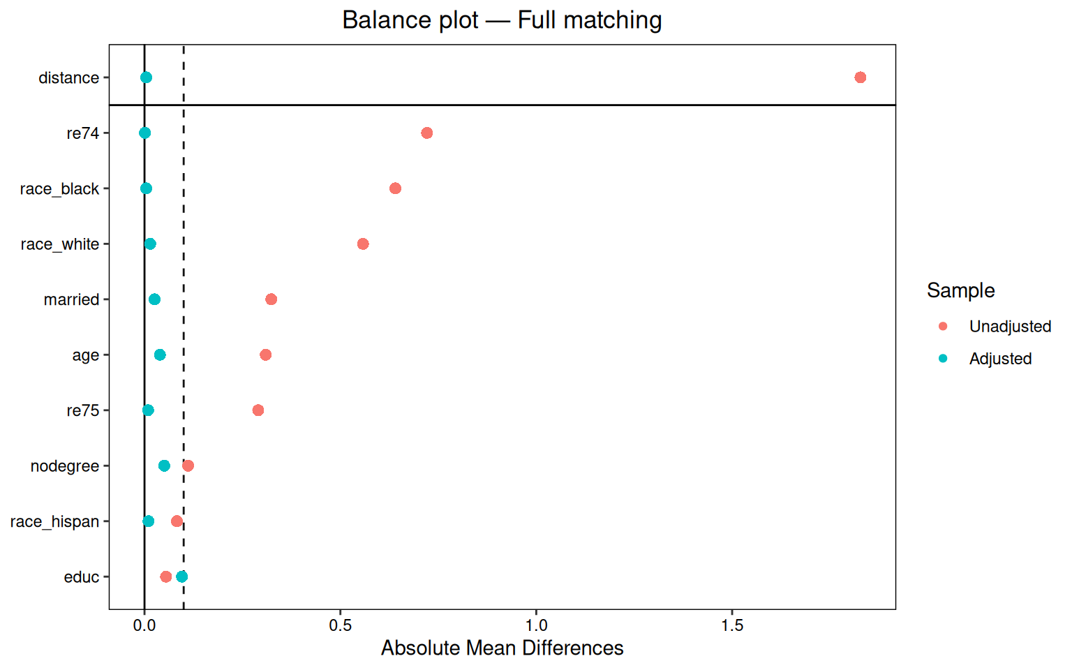
A useful rule is that standardized mean differences should be below 0.1, or below 0.05 if we want to be stricter.
7.7 Matching with replacement vs without
By default a control observation can be used only once. With replacement, the same good control can be used several times. This often improves balance when overlap is weak, but the effective sample size becomes smaller.
Balance Measures
                Type Diff.Adj        M.Threshold
distance    Distance   0.0044     Balanced, <0.1
age          Contin.   0.2395 Not Balanced, >0.1
educ         Contin.  -0.0161     Balanced, <0.1
race_black    Binary   0.0054     Balanced, <0.1
race_hispan   Binary  -0.0054     Balanced, <0.1
race_white    Binary   0.0000     Balanced, <0.1
married       Binary   0.0595     Balanced, <0.1
nodegree      Binary   0.0054     Balanced, <0.1
re74         Contin.  -0.0493     Balanced, <0.1
re75         Contin.   0.0087     Balanced, <0.1

Balance tally for mean differences
                   count
Balanced, <0.1         9
Not Balanced, >0.1     1

Variable with the greatest mean difference
 Variable Diff.Adj        M.Threshold
      age   0.2395 Not Balanced, >0.1

Sample sizes
                     Control Treated
All                   429.       185
Matched (ESS)          46.31     185
Matched (Unweighted)   82.       185
Unmatched             347.         0
If matching without replacement cannot balance the sample, matching with replacement is a reasonable next step.
7.8 ATE, ATT, ATC — choose carefully
MatchIt usually targets the ATT. That means we are asking what treatment did for the treated units. For ATE, use estimand = "ATE" and a method that keeps the whole sample, such as full matching or weighting. For ATC, use estimand = "ATC". These are not just software options; they are different causal questions.
7.9 When matching fails
Matching fails in predictable ways:
- High-dimensional matching is hard. Propensity scores reduce dimension, but they do not create overlap.
- If some values of \(X\) have no treated or no control units, no matching method can recover the missing comparison.
- Propensity-score matching depends on the propensity-score model. If that model is bad, the matching can be bad too.
- Matching does not address hidden confounding. Rosenbaum bounds, discussed in the Sensitivity Analysis chapter, ask how strong hidden bias would have to be to change the conclusion.
7.10 Matching vs weighting
Matching and weighting do similar jobs. Matching chooses comparable observations. Weighting keeps observations but changes their contribution so the treated and control covariate distributions become closer.
When overlap is good, both approaches often give similar answers. When overlap is bad, both approaches become fragile. Then the honest choices are to change the target population, report the lack of overlap, or use a doubly-robust estimator such as AIPW or TMLE while still being clear about the support problem.
7.11 Weighting Alternatives
WeightIt implements several weighting methods. The companion blog chapter on weighting has more detail. Here I use the same Lalonde data so the comparison is easy.
7.11.1 Inverse probability of treatment weighting (IPW)
The baseline method is IPW. Estimate the propensity score, then weight by the inverse probability of receiving the observed treatment.
Balance Measures
                Type Diff.Adj         M.Threshold
prop.score  Distance  -0.0205     Balanced, <0.05
age          Contin.   0.1188 Not Balanced, >0.05
educ         Contin.  -0.0284     Balanced, <0.05
race_black    Binary  -0.0022     Balanced, <0.05
race_hispan   Binary   0.0002     Balanced, <0.05
race_white    Binary   0.0021     Balanced, <0.05
married       Binary   0.0186     Balanced, <0.05
nodegree      Binary   0.0184     Balanced, <0.05
re74         Contin.  -0.0021     Balanced, <0.05
re75         Contin.   0.0110     Balanced, <0.05

Balance tally for mean differences
                    count
Balanced, <0.05         9
Not Balanced, >0.05     1

Variable with the greatest mean difference
 Variable Diff.Adj         M.Threshold
      age   0.1188 Not Balanced, >0.05

Effective sample sizes
           Control Treated
Unadjusted  429.       185
Adjusted     99.82     185
7.11.2 Covariate balancing propensity score (CBPS)
CBPS estimates the propensity score while also trying to balance covariate means. So the propensity-score model is not judged only by likelihood; it is also judged by balance.
Balance Measures
                Type Diff.Adj     M.Threshold
prop.score  Distance   -0.018 Balanced, <0.05
age          Contin.    0.000 Balanced, <0.05
educ         Contin.   -0.000 Balanced, <0.05
race_black    Binary   -0.000 Balanced, <0.05
race_hispan   Binary   -0.000 Balanced, <0.05
race_white    Binary    0.000 Balanced, <0.05
married       Binary   -0.000 Balanced, <0.05
nodegree      Binary   -0.000 Balanced, <0.05
re74         Contin.   -0.000 Balanced, <0.05
re75         Contin.   -0.000 Balanced, <0.05

Balance tally for mean differences
                    count
Balanced, <0.05        10
Not Balanced, >0.05     0

Variable with the greatest mean difference
 Variable Diff.Adj     M.Threshold
     re74       -0 Balanced, <0.05

Effective sample sizes
           Control Treated
Unadjusted  429.       185
Adjusted     98.46     185
7.11.3 Entropy balancing
Entropy balancing chooses weights so that the weighted control group matches the treated group on covariate means. It is useful because the balance constraint is explicit.
Balance Measures
               Type Diff.Adj     M.Threshold
age         Contin.       -0 Balanced, <0.05
educ        Contin.       -0 Balanced, <0.05
race_black   Binary        0 Balanced, <0.05
race_hispan  Binary        0 Balanced, <0.05
race_white   Binary       -0 Balanced, <0.05
married      Binary       -0 Balanced, <0.05
nodegree     Binary        0 Balanced, <0.05
re74        Contin.       -0 Balanced, <0.05
re75        Contin.       -0 Balanced, <0.05

Balance tally for mean differences
                    count
Balanced, <0.05         9
Not Balanced, >0.05     0

Variable with the greatest mean difference
 Variable Diff.Adj     M.Threshold
     re74       -0 Balanced, <0.05

Effective sample sizes
           Control Treated
Unadjusted  429.       185
Adjusted     98.46     185
The standardized mean differences are essentially zero because entropy balancing imposes mean balance directly.
7.11.4 Energy balancing
Energy balancing targets the whole covariate distribution, not just means. It is more ambitious than entropy balancing, and usually more computationally expensive.
Balance Measures
               Type Diff.Adj     M.Threshold
age         Contin.  -0.0016 Balanced, <0.05
educ        Contin.   0.0106 Balanced, <0.05
race_black   Binary   0.0060 Balanced, <0.05
race_hispan  Binary  -0.0008 Balanced, <0.05
race_white   Binary  -0.0053 Balanced, <0.05
married      Binary  -0.0011 Balanced, <0.05
nodegree     Binary   0.0050 Balanced, <0.05
re74        Contin.  -0.0021 Balanced, <0.05
re75        Contin.   0.0226 Balanced, <0.05

Balance tally for mean differences
                    count
Balanced, <0.05         9
Not Balanced, >0.05     0

Variable with the greatest mean difference
 Variable Diff.Adj     M.Threshold
     re75   0.0226 Balanced, <0.05

Effective sample sizes
           Control Treated
Unadjusted  429.       185
Adjusted     41.82     185
7.11.5 Estimation with weighted-aware regression
After computing weights, use lm_weightit() instead of plain lm if we want standard errors that account for the estimated weights.
fit_ebal <- lm_weightit(
  re78 ~ treat * (age + educ + race + married + nodegree + re74 + re75),
  data     = lalonde,
  weightit = w_ebal
)

avg_comparisons(fit_ebal, variables = "treat",
                newdata = subset(lalonde, treat == 1))   # ATT
 Estimate Std. Error    z Pr(>|z|)   S 2.5 % 97.5 %
     1273        770 1.65   0.0983 3.3  -236   2783

Term: treat
Type: probs
Comparison: 1 - 0
This gives the entropy-balanced ATT and a sandwich-style standard error.
7.11.6 When to use each weighting method
| Method | Strengths | Weaknesses |
|---|---|---|
| IPW (glm) | Familiar; well-studied | Sensitive to PS misspecification; extreme weights |
| CBPS | Balance-constrained PS; robust to model misspecification | Slower; can fail with many covariates |
| Entropy balancing | Exact mean balance; doubly robust for ATT | Balances means only, not distributions |
| Energy balancing | Balances entire distribution | Computationally heavier; less mature theory |
For applied work, entropy balancing is often a good default because it is simple and the balance diagnostics are easy to explain. Energy balancing is useful when matching the whole covariate distribution is important.
7.11.7 Comparing matching to weighting
The matching and weighting examples here target the same ATT. In an applied paper I would report balance for each method, not just the final coefficient. If several reasonable methods give similar balance and similar estimates, the result is more credible. If they differ sharply, the problem is usually weak overlap or model dependence.
For more details on MatchIt and the Stata teffects commands, see the matching blog chapter and treatment-effects in Stata.
7.12 Summary
- Matching is for selection on observables. It does not fix unobserved confounding.
- The main diagnostic is covariate balance, not the treatment-effect coefficient.
- Propensity-score matching is simple, but full matching or weighting often balances better.
- If there is no overlap, change the estimand or restrict the sample. Do not hide the support problem.