1 Identification & Potential Outcomes
1.1 Why Do We Need Tools for Causal Inference?
Association is not causation. We have known how to measure associations for a long time, but most econometric models are associational. The gap between the two arises from confounding.
1.2 Confounders
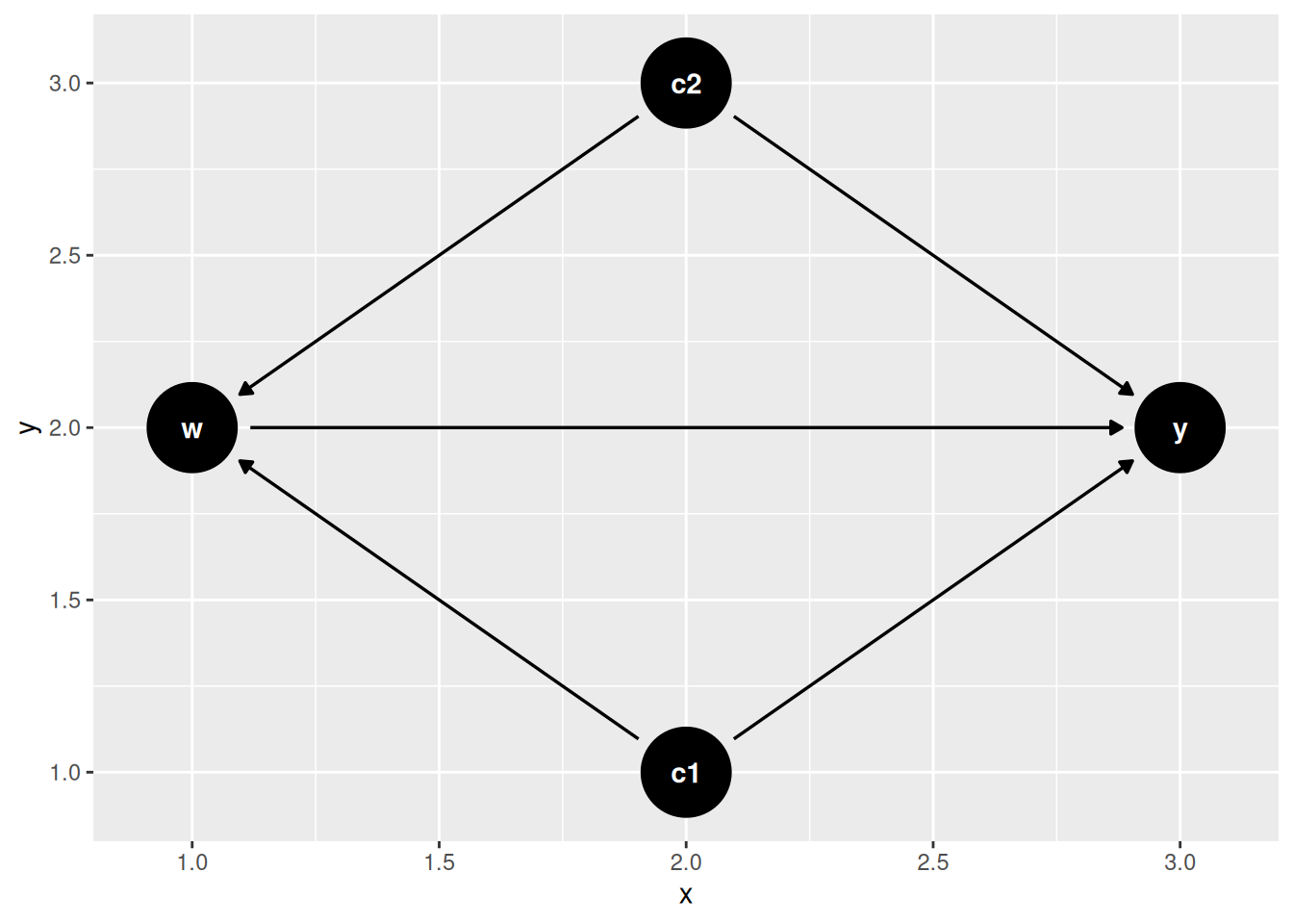
The graphical language used throughout this book is Pearl’s (2009). In this graph, \(w\) is the treatment, \(y\) the outcome, and \(c_1\), \(c_2\) are confounders. Both confounders affect both \(w\) and \(y\), so the observed association between \(w\) and \(y\) may reflect confounding rather than a causal effect.
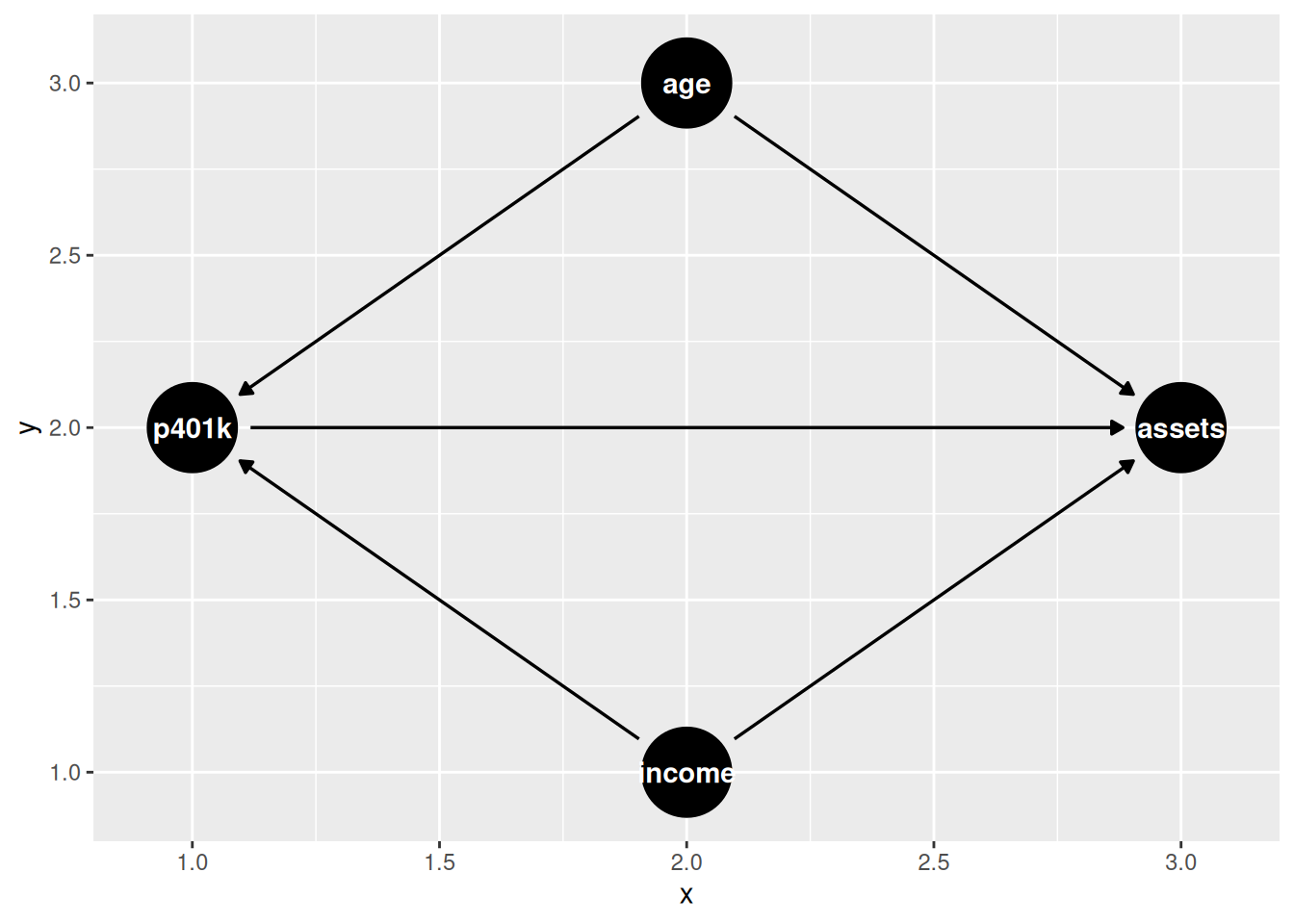
A concrete example: income and age may both drive 401(k) participation and assets. To identify the causal effect of participation on assets, we need to control for income and age.
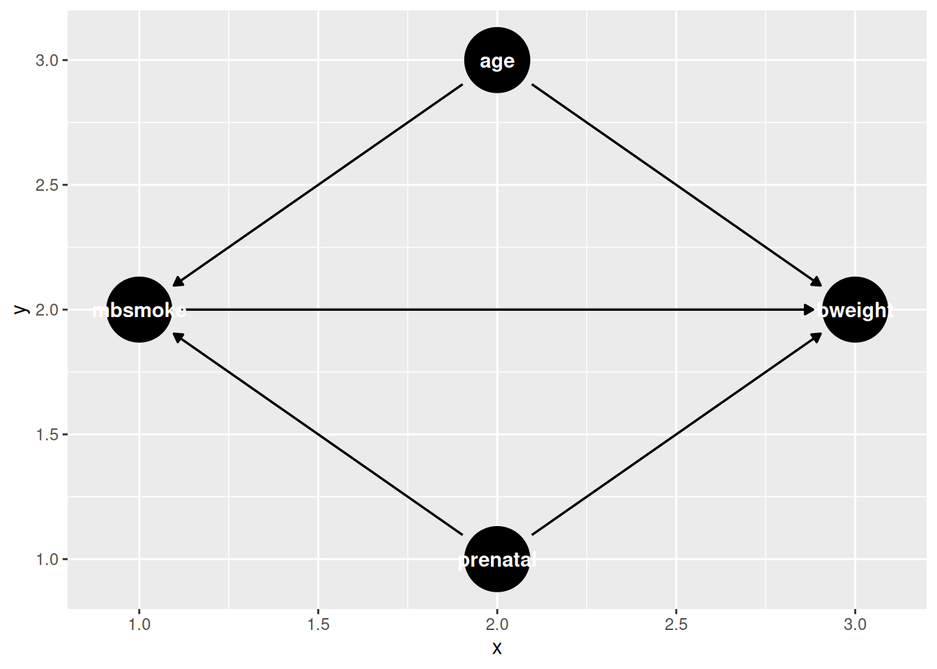
And another example with birth weight and maternal smoking. It could be the case that prenatal care and maternal age are causing both maternal smoking and birth weight. It could be that maternal smoking has nothing to do with birth weight. But age and prenatal care are causing both maternal smoking and birth weight, therefore maternal smoking appears to cause birth weight.
1.3 Controlled and Uncontrolled Confounders
If we can control for all confounders, correlation comes close to implying causation – but adjustment alone does not finish the job. It has to be joined by the conditions set out below: consistency, positivity, and no interference, along with adjusting on the right set and estimating it correctly. Controlling for confounders is necessary, not sufficient. Two questions follow from it: do we observe all confounders, and how do we control for them? In a randomized experiment neither arises. In an observational study both do.
If \(c_2\) is unobserved, adjusting on the observed covariates will not recover the effect of \(w\) on \(y\). That is a statement about backdoor adjustment, not about the effect being beyond reach: instrumental variables, front-door adjustment, regression discontinuity and panel designs can each identify an effect in the presence of an unmeasured common cause, and the rest of this book develops them.
1.4 Potential Outcome Setup
We study causal effects through the potential outcomes (counterfactual) framework, introduced by Neyman (1990) for randomized experiments and extended to observational studies by Rubin (1974). Each unit has two potential outcomes, \(Y(1)\) and \(Y(0)\), one for each treatment state. These are fixed before any assignment; the experiment tries to recover them. The fundamental problem of causal inference (Holland 1986) is that we never observe both: only the realized outcome \(Y = WY(1) + (1-W)Y(0)\) is seen. Individual treatment effects \(\tau_i = Y_i(1) - Y_i(0)\) are not identifiable; only averages can be estimated.
We write \(W\) for treatment assignment and \(X\) for covariates.
1.5 ATE, ATT and ATU
The standard estimands, in the taxonomy Imbens (2004) uses to organise this literature, are:
\[ \tau_{ATE} = E[Y(1) - Y(0)] \tag{1.1}\]
\[ \tau_{ATT} = E[Y(1) - Y(0) | W=1] \tag{1.2}\]
\[ \tau_{ATU} = E[Y(1) - Y(0)| W=0] \tag{1.3}\]
\[ \tau_{ATE} = \rho \tau_{ATT} + (1-\rho) \tau_{ATU} \tag{1.4}\]
where \(\rho= P(W=1)\).
1.6 Identification: From Potential Outcome to Observed
We focus on \(\tau_{ATT}\). To identify it, we need: \[ E[Y(1) | W=1] \tag{1.5}\] which is easy, because we observe it.
And we need \[ E[Y(0) | W=1] \tag{1.6}\]
To identify this, we’ll need unconfoundedness: \[ E[Y(0) | W, X] = E[Y(0)| X] \tag{1.7}\] and overlap: \[ \pi(x)= P(W=1 | X=x) < 1 \tag{1.8}\] (for the ATT only \(\pi(x)<1\) is needed; the ATE requires \(0<\pi(x)<1\)).
Unconfoundedness says that within each subgroup \(X=x\), treated and control units have the same mean of \(Y(0)\): \(E[Y(0)|W=1,X=x]=E[Y(0)|W=0,X=x]=E[Y|W=0,X=x]\). Averaging over the covariate distribution of the treated,
\[ E[Y(0)| W=1] = E\big[ E[Y | W=0, X] \mid W=1 \big], \tag{1.9}\]
which involves only observed data. Therefore ATT is identified:
\[ \begin{aligned} \tau_{ATT} &= E[Y(1) - Y(0) | W=1] \\ &= E[Y|W=1] - E\big[ E[Y | W=0, X] \mid W=1 \big] \end{aligned} \tag{1.10}\]
Note the conditional-on-\(X\) assumption does NOT imply the marginal equality \(E[Y(0)|W=1]=E[Y(0)|W=0]\): treated and control units have different covariate distributions, so the adjustment over \(X\) is essential. In a randomised experiment, unconfoundedness holds without conditioning on \(X\) (i.e. \(E[Y(0)|W]=E[Y(0)]\)); then \(E[Y(0)|W=1]=E[Y(0)|W=0]=E[Y|W=0]\), the formula collapses to \(E[Y|W=1]-E[Y|W=0]\), and a difference-in-means estimator is consistent.
\[ \hat{\tau}_{ATT} = \bar Y_1 - \bar Y_0 \tag{1.11}\]
In observational studies, unconfoundedness is rarely credible without further justification. The rest of this book develops the tools for doing so.
1.7 Unconfoundedness and Overlap
Weaker Assumptions: Unconfoundedness (conditional independence, or ignorability, in the sense of Rosenbaum and Rubin (1983)), stated jointly for both potential outcomes since we are after the ATE here (as opposed to the ATT case above, which only required it for \(Y(0)\)): \[ E[Y(d) | W, X] = E[Y(d)| X] \quad \text{for } d \in \{0,1\} \tag{1.12}\] Overlap: \[ 0 < \pi(x)= P(W=1 | X=x) < 1 \tag{1.13}\] SUTVA (stable unit treatment value assumption, Rubin (1974); see Imbens and Rubin (2015) for a book-length treatment): 1. No interference between units. No spillovers. 2. Consistency. No hidden versions of treatment or control. Treatment is clearly defined.
Within each subgroup of \(X=x\), W is independent of \(Y(0)\). With the overlap assumption, we ensure there is a comparable control unit for each treated unit.
However, these two criteria are often contradictory: we may need more covariates to satisfy conditional independence; meanwhile, if the dimension of covariates goes high, then it’s likely in some partition we don’t have control units.
We need four assumptions for identification:
- Unconfoundedness (conditional independence, or ignorability)
- Overlap (positivity, common support)
- No interference
- Consistency
1.8 Observational Data Flowchart
In observational studies, this is the map I keep in mind – which designs are available, and what each one asks you to assume:
%%{init: {'flowchart': {'diagramPadding': 30}}}%%
flowchart LR
  A[Observational data Y,W,X] --> B{Unconfoundedness?}
  B --> | Yes | C{Nuisance models: parametric or flexible/ML?}
  C --> | Parametric | D(RA)
  C --> | Parametric | E(IPW)
  C --> | Parametric | F(AIPW)
  C --> | Parametric | G(IPWRA)
  C --> | Flexible/ML with cross-fitting | H(AIPW)
  C --> | Flexible/ML with cross-fitting | I(TMLE)
  C --> | Flexible/ML with cross-fitting | J(DoubleML)
  B --> | No | K{Panel data?}
  K --> | Yes | L{Parallel Trend?}
  L --> | Yes | M(DID)
  L --> | No, but factor structure and pre-period fit | N(Synthetic Control)
  L --> | No, but factor structure and pre-period fit | O(Synthetic DID)
  K --> | No | P{Assignment rule?}
  P --> | Cutoff, with continuity at the threshold | Q2(RDD)
  P --> | Instrument, relevant and excludable | Q(IV)
  P --> | Neither | R(Bounds and sensitivity analysis)
Read that as a map of designs and their assumptions, not as a decision rule. None of the branches is an assumption-free repair; each trades one assumption for another. Synthetic control and synthetic DiD do not dispense with a counterfactual assumption when parallel trends fails – they replace it with a factor structure and a stability condition, which the pre-period fit is meant to make credible rather than to prove. Regression discontinuity replaces unconfoundedness with continuity of potential outcomes at the cutoff, which is why it needs its own branch rather than sharing one with instrumental variables. And the last box is not quite a dead end: when no design identifies the effect, bounds and sensitivity analysis are what remain, and the sensitivity analysis chapter takes them up.