    year countyreal     lpop     lemp first.treat treat
866 2003       8001 5.896761 8.461469        2007     1
841 2004       8001 5.896761 8.336870        2007     1
842 2005       8001 5.896761 8.340217        2007     1
819 2006       8001 5.896761 8.378161        2007     1
827 2007       8001 5.896761 8.487352        2007     1
937 2003 8019 2.232377 4.997212 2007 112 Difference-in-Differences
What if unconfoundedness fails? We have to settle for weaker assumptions. One such assumption is the parallel trends assumption. If we have this assumption, we can use a difference-in-differences estimator.
Related reading: For a side-by-side comparison of DiD, synthetic control, synthetic DiD, and multivariate SC on a single panel — and how the choice of estimator changes the answer — see the Same data, different estimators chapter in Topics on Econometrics and Causal Inference.
12.1 \(T=2\) Panel Data
Suppose we have two periods, \(t = (1,2)\). Some units are treated just prior to period 2. For each individual \(i\), there are four potential outcomes:
\[ [Y_{i1}(0), Y_{i1}(1), Y_{i2}(0), Y_{i2}(1)] \]
We use \(D\) to identify the treated group.
The ATT when \(T=2\):
\[ \tau_{2,att} = E(Y_2(1) - Y_2(0) | D=1) \]
In words, we are interested in the ATT in the second period. The difficult part is the second term.
12.2 Parallel Trends Assumption
\[ E[Y_2(0) -Y_1(0) | D=1] = E[Y_2(0) - Y_1(0) | D =0] \]
or
\[ E[\Delta Y(0) | D=1] = E[\Delta Y(0) | D =0] \]
In other words, this means the change of potential outcome for untreated state between period 1 and 2 is independent of treatment assignment (unconfounded).
12.3 No Anticipation Assumption
\[ E[Y_1(1) - Y_1(0) | D=1] = 0 \]
This is to say, in period 1, there is no treatment effect for the treated group.
12.4 DiD is Identified with PT and NA
With Parallel Trends, we notice \[\small E[Y_2(0) | D=1 ]= E[Y_1(0) | D=1] + E[Y_2(0) - Y_1(0) | D=0] \]
Then, with No Anticipation, \[\small \begin{align} E[Y_2(0) | D=1 ] &= E[Y_1(1) | D=1] + E[Y_2(0) - Y_1(0) | D=0]\\ &= E[Y_1 | D=1] + E[Y_2-Y_1 | D=0] \end{align} \]
\[\small \tau_{2,att} = E[Y_2 - Y_1 | D=1] - E[Y_2-Y_1 | D=0] \]
12.5 Advantages and Disadvantages of DiD
Advantages:
- No need to assume unconfoundedness. We “only” need PT and NA. Or say we don’t need treatment itself to be independent of potential outcomes, but we do need it to be independent to the change in potential outcome at least for untreated state. This is importantly weaker in a lot of situations. There can be selection bias. If the selection bias does not change over time, then DiD can handle it.
Disadvantages:
- PT and NA might be violated.
- PT is not scale free, in the sense that even if outcome can have PT, but then non-linear transformation of outcome won’t have PT (for example log of Y).
12.6 Traditional DiD
In practice, DiD in many period setting is usually done with
\[ Y_{it} = \alpha_i + \phi_t + W_{it} \beta + \epsilon_{it} \]
here \(W_{it} =(1[t=2] \cdot D_i)\), which is the interaction of post-treatment indicator and treatment group indicator.
This is usually called Two Way Fixed Effect (TWFE). There are multiple ways to implement the same model in practice.
TWFE can be done by “Pooled OLS”. That is, using OLS on time dummies and firm (individual) dummies. Wooldridge (2021) shows it’s equivalent to use treatment dummies, instead of individual dummies. He also shows that this model can be equivalently implemented with fixed effect model and random effect model.
12.7 TWFE with Staggered Treatment Timing
The problem comes in when there is different timing of treatment. People used to still use
\[ Y_{it} = \alpha_i + \phi_t + W_{it} \beta + \epsilon_{it} \]
where \(W_{it}\) now is a dummy when an individual \(i\) gets treated at time \(t\).
However, what is \(\beta\) here?
12.8 Goodman-Bacon Decomposition
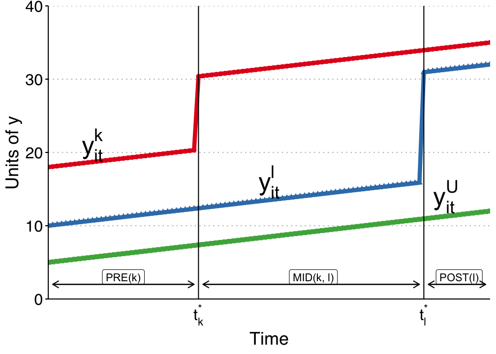
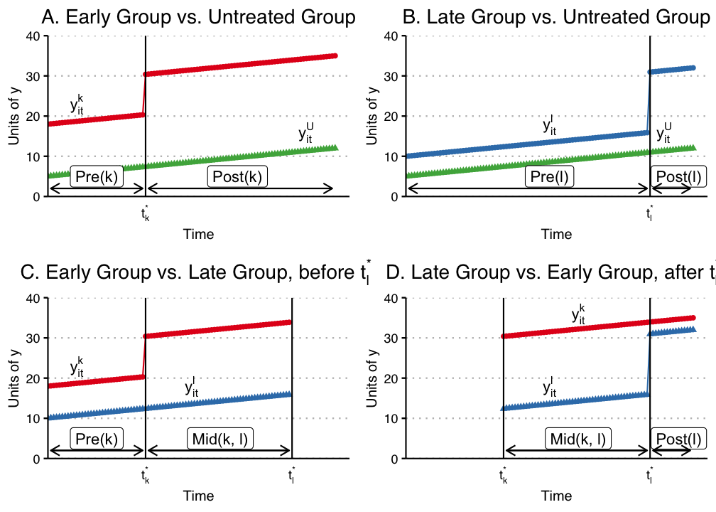
Goodman-Bacon (2021) showed that \(\beta\) in the TWFE is a weighted average of many different treatment effects, between treated cohorts, and control units, both can be different at different time points. The weights are a function of the size of the subsample, relative size of treatment and control units, and the timing of treatment in the sub sample. The decomposition weights themselves are non-negative and sum to one; the problem is that the units treated earlier are used as controls later. When those “forbidden” 2x2 comparisons are expressed in terms of the underlying cohort-time ATTs, some ATTs receive negative weight (de Chaisemartin and D’Haultfœuille 2020). Therefore there is no meaningful interpretation of \(\beta\): it does not need to be a convex combination of treatment effects.
12.9 Wooldridge’s ETWFE
There are a lot of ways to deal with staggered DiD situation. Wooldridge (2021) is basically saying: This is not a problem of TWFE, it’s a mis-use of TWFE. The reason we get non-sensible result of \(\beta\) is that we know there is heterogeneous treatment effect, in the sense the treatment effect differs across cohort, but we force them to be the same. If we relax it, it can work. As he shows, this works when we specify cohort effects accordingly.
\[ y_{it} = \alpha_i + \phi_t + \sum_{g=g_0}^G \sum_{t=g}^T \lambda_{g,t} \times 1(g,t) + \epsilon_{i,t} \]
Here \(g\) is a cohort indicator, a cohort is determined by the time of getting treatment. ETWFE is allowing each cohort to have different effect at each different time point after being treated. The baseline group is the never treated group. If there is no never treated group, it can easily be changed to comparing to the last treated group.
12.10 Example 1: US Teen Employment
We’ll use the mpdta dataset on US teen employment from the did package. “Treatment” in this dataset refers to an increase in the minimum wage rate. Our goal is to estimate the effect of this minimum wage treatment (treat) on the log of teen employment (lemp). Notice that the panel ID is at the county level (countyreal), but treatment was staggered across cohorts (first.treat) so that a group of counties were treated at the same time. In addition to these staggered treatment effects, we also observe log population (lpop) as a potential control variable.
table(mpdta$year)
2003 2004 2005 2006 2007
500 500 500 500 500 table(mpdta$treat)
   0    1
1545 955 table(mpdta$first.treat)
   0 2004 2006 2007
1545 100 200 655 modOLS estimation, Dep. Var.: lemp
Observations: 2,500
Fixed-effects: first.treat: 4, year: 5
Standard-errors: Clustered (countyreal)
Estimate Std. Error t value Pr(>|t|)
lpop 1.065461 0.021824 48.821102 < 2.2e-16 ***
first.treat::2004:lpop 0.050982 0.037756 1.350320 0.177525
first.treat::2006:lpop -0.041095 0.047390 -0.867183 0.386259
first.treat::2007:lpop 0.055518 0.039212 1.415838 0.157447
year::2004:lpop 0.011014 0.007554 1.458043 0.145458
year::2005:lpop 0.020733 0.008104 2.558268 0.010814 *
year::2006:lpop 0.010535 0.010816 0.974084 0.330487
year::2007:lpop 0.020921 0.011808 1.771708 0.077053 .
... 14 coefficients remaining (display them with summary() or use
argument n)
... 10 variables were removed because of collinearity
(.Dtreat:first.treat::2006:year::2004,
.Dtreat:first.treat::2006:year::2005 and 8 others [full set in
$collin.var])
---
Signif. codes: 0 '***' 0.001 '**' 0.01 '*' 0.05 '.' 0.1 ' ' 1
RMSE: 0.537131 Adj. R2: 0.871722
Within R2: 0.869464emfx(mod)
 .Dtreat Estimate Std. Error     z Pr(>|z|)    S   2.5 %  97.5 %
    TRUE  -0.0506     0.0125 -4.05   <0.001 14.3 -0.0751 -0.0261

Term: .Dtreat
Type: response
Comparison: TRUE - FALSE
mod_es = emfx(mod, type = "event")
mod_es
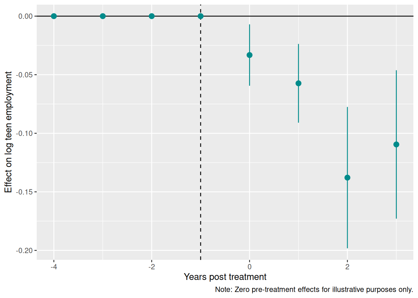
 event Estimate Std. Error     z Pr(>|z|)    S   2.5 %   97.5 %
     0  -0.0332     0.0134 -2.48    0.013  6.3 -0.0594 -0.00702
     1  -0.0573     0.0171 -3.34   <0.001 10.2 -0.0910 -0.02373
     2  -0.1379     0.0308 -4.48   <0.001 17.0 -0.1982 -0.07753
     3  -0.1095     0.0323 -3.39   <0.001 10.5 -0.1729 -0.04620

Term: .Dtreat
Type: response
Comparison: TRUE - FALSE
mod_es2 = emfx(mod, type = "event", post_only = FALSE)
ggplot(mod_es2, aes(x = event, y = estimate, ymin = conf.low, ymax = conf.high)) +
geom_hline(yintercept = 0) +
geom_vline(xintercept = -1, lty = 2) +
geom_pointrange(col = "darkcyan") +
labs(
x = "Years post treatment", y = "Effect on log teen employment",
caption = "Note: Zero pre-treatment effects for illustrative purposes only."
)
12.11 Example 2: Staggered DiD
# A tibble: 6 × 11
     id  year     y     x    d4    d5    d6   te4   te5   te6 first_treat
  <dbl> <dbl> <dbl> <dbl> <dbl> <dbl> <dbl> <dbl> <dbl> <dbl>       <dbl>
1     1  2001  18.4 0.900     0     0     0  0     0    0               0
2     1  2002  18.1 0.900     0     0     0  0     0    0               0
3     1  2003  18.6 0.900     0     0     0  0     0    0               0
4     1  2004  16.5 0.900     0     0     0  1.43  0    0               0
5     1  2005  20.0 0.900     0     0     0  2.57  2.25 0               0
6 1 2006 19.9 0.900 0 0 0 5.07 4.23 0.786 0table(did_data$first_treat)
   0 2004 2005 2006
1572  714  498  216
did_data <- did_data %>%
mutate(treated_cohort1 = case_when(d4 & f04 ~ "d4f04",
d4 & f05 ~ "d4f05",
d4 & f06 ~ "d4f06"),
treated_cohort2 = case_when (
d5 & f05 ~ "d5f05",
d5 & f06 ~ "d5f06"),
treated_cohort3= case_when(
d6 & f06 ~ "d6f06"))
did_data %>%
group_by(treated_cohort1) %>%
summarise(mean4=mean(te4))# A tibble: 4 × 2
treated_cohort1 mean4
<chr> <dbl>
1 d4f04 3.76
2 d4f05 4.02
3 d4f06 4.58
4 <NA> 1.83 did_data %>%
group_by(treated_cohort2) %>%
summarise(mean5=mean(te5))# A tibble: 3 × 2
treated_cohort2 mean5
<chr> <dbl>
1 d5f05 2.74
2 d5f06 3.52
3 <NA> 0.978 did_data %>%
group_by(treated_cohort3) %>%
summarise(mean6=mean(te6))# A tibble: 2 × 2
treated_cohort3 mean6
<chr> <dbl>
1 d6f06 1.85
2 <NA> 0.329OLS estimation, Dep. Var.: y
Observations: 3,000
Fixed-effects: first_treat: 4, year: 6
Standard-errors: Clustered (id)
Estimate Std. Error t value Pr(>|t|)
x 0.240952 0.452664 0.532298 0.5947564
first_treat::2004:x -1.191253 0.934130 -1.275254 0.2028127
first_treat::2005:x 0.551133 0.606947 0.908042 0.3642944
first_treat::2006:x 0.994478 0.827570 1.201685 0.2300556
year::2002:x 0.395894 0.327576 1.208558 0.2274050
year::2003:x 0.975554 0.319476 3.053604 0.0023818 **
year::2004:x 0.330593 0.350924 0.942064 0.3466155
year::2005:x 0.238847 0.398165 0.599869 0.5488659
... 13 coefficients remaining (display them with summary() or use
argument n)
... 18 variables were removed because of collinearity
(.Dtreat:first_treat::2004:year::2002,
.Dtreat:first_treat::2004:year::2003 and 16 others [full set in
$collin.var])
---
Signif. codes: 0 '***' 0.001 '**' 0.01 '*' 0.05 '.' 0.1 ' ' 1
RMSE: 2.92391 Adj. R2: 0.194759
Within R2: 0.110397emfx(mod)
 .Dtreat Estimate Std. Error    z Pr(>|z|)     S 2.5 % 97.5 %
    TRUE     3.67      0.172 21.3   <0.001 333.2  3.33   4.01

Term: .Dtreat
Type: response
Comparison: TRUE - FALSE
mod_es = emfx(mod, type = "event")
mod_es
 event Estimate Std. Error    z Pr(>|z|)     S 2.5 % 97.5 %
     0     3.11      0.213 14.6   <0.001 158.5  2.69   3.53
     1     4.02      0.248 16.2   <0.001 193.4  3.53   4.51
     2     4.21      0.331 12.7   <0.001 120.9  3.56   4.86

Term: .Dtreat
Type: response
Comparison: TRUE - FALSE
mod_es2 = emfx(mod, type = "calendar")
mod_es2
 year Estimate Std. Error    z Pr(>|z|)     S 2.5 % 97.5 %
 2004     3.51      0.303 11.6   <0.001 100.6  2.92   4.10
 2005     3.73      0.253 14.7   <0.001 160.9  3.24   4.23
 2006     3.70      0.249 14.8   <0.001 163.0  3.21   4.19

Term: .Dtreat
Type: response
Comparison: TRUE - FALSE
12.12 Nonlinear ETWFE: Count and Binary Outcomes
ETWFE is not limited to linear (continuous) outcomes. When the dependent variable is a count or a binary indicator, linear TWFE can give nonsensical results — negative predicted probabilities, additive effects that ignore the bounded or non-negative nature of \(Y\). The etwfe package supports nonlinear families via the family argument, which passes to fixest::feglm().
The key identifying assumption shifts slightly. Instead of parallel trends on \(E[Y_{it}(\infty)]\), we assume parallel trends on the linear index — that is, on \(\log E[Y_{it}(\infty)]\) for Poisson, or on \(\text{logit}\, E[Y_{it}(\infty)]\) for logit. This is Wooldridge’s (2023) Conditional Parallel Trends assumption stated on \(G^{-1}(E[Y])\). When the true treatment effect is multiplicative (e.g., a policy raises counts by 50% regardless of baseline), this assumption is more natural than additive PT on \(Y\) itself.
One implementation detail matters: the nonlinear ETWFE specification uses cohort fixed effects (one intercept per treatment cohort) plus year fixed effects — not individual unit fixed effects. The etwfe package handles this automatically. In the linear case the two are numerically equivalent (Wooldridge 2021), but in nonlinear models unit fixed effects raise the incidental-parameters problem and make average partial effects uncomputable — the unit intercepts cannot be averaged out of the nonlinear link. Wooldridge (2023) instead uses cohort intercepts (a Mundlak device), which is what etwfe implements.
12.12.1 Simulated example: staggered count data
We simulate panel data with three treatment cohorts (treated in periods 3, 4, and 5) and one never-treated group. The true treatment effect is multiplicative: treated units see a 50% increase in their expected count (\(\exp(0.4) - 1 \approx 0.49\)). Parallel trends holds on the log scale.
library(tidyverse)
library(etwfe)

set.seed(42)
N <- 400; Tmax <- 6

unit_fe_vals <- rnorm(N) * 0.3

df_count <- expand.grid(id = 1:N, year = 1:Tmax) %>%
  as_tibble() %>%
  arrange(id, year) %>%
  mutate(
    cohort_grp  = ((id - 1) %/% 100) + 1,
    first_treat = c(3, 4, 5, 0)[cohort_grp],   # 0 = never treated
    treated     = (first_treat > 0) & (year >= first_treat),
    unit_fe     = unit_fe_vals[id],
    log_mu      = 1 + 0.2 * year + unit_fe + 0.4 * treated,
    count       = rpois(n(), exp(log_mu))
  )

df_count %>%
  group_by(first_treat, treated) %>%
  summarise(mean_count = mean(count), .groups = "drop")
# A tibble: 7 × 3
first_treat treated mean_count
<dbl> <lgl> <dbl>
1 0 FALSE 6.15
2 3 FALSE 3.72
3 3 TRUE 10.7
4 4 FALSE 4.29
5 4 TRUE 11.5
6 5 FALSE 4.80
7 5 TRUE 13.2 12.12.2 Poisson ETWFE
Pass family = "poisson" to etwfe(). Everything else — cohort dummies, emfx(), event study — works identically to the linear case. We use cgroup = "never" so that pre-treatment estimates are not mechanistically forced to zero.
mod_pois <- etwfe(
  fml         = count ~ 1,
  tvar        = year,
  gvar        = first_treat,
  data        = df_count,
  family      = "poisson",
  cgroup      = "never",
  vcov        = ~id
)emfx(mod_pois)
 .Dtreat Estimate Std. Error    z Pr(>|z|)     S 2.5 % 97.5 %
    TRUE     3.99       0.33 12.1   <0.001 109.6  3.34   4.64

Term: .Dtreat
Type: response
Comparison: TRUE - FALSE
emfx() returns average marginal effects — the average difference \(E[Y(1)] - E[Y(0)]\) in count units across treated observations. This is the ATT on the count scale. The underlying model imposes PT on the log scale, so each cohort-time treatment coefficient in the raw model can be exponentiated to get the incidence rate ratio for that cell (here they share a common value because the simulated effect is homogeneous).
12.12.3 Event study
mod_pois_es <- emfx(mod_pois, type = "event", post_only = FALSE)

ggplot(mod_pois_es, aes(x = event, y = estimate, ymin = conf.low, ymax = conf.high)) +
  geom_hline(yintercept = 0) +
  geom_vline(xintercept = -1, lty = 2) +
  geom_pointrange(col = "darkcyan") +
  labs(
    x = "Years post treatment",
    y = "ATT (count units)",
    title = "Nonlinear ETWFE event study (Poisson)"
  )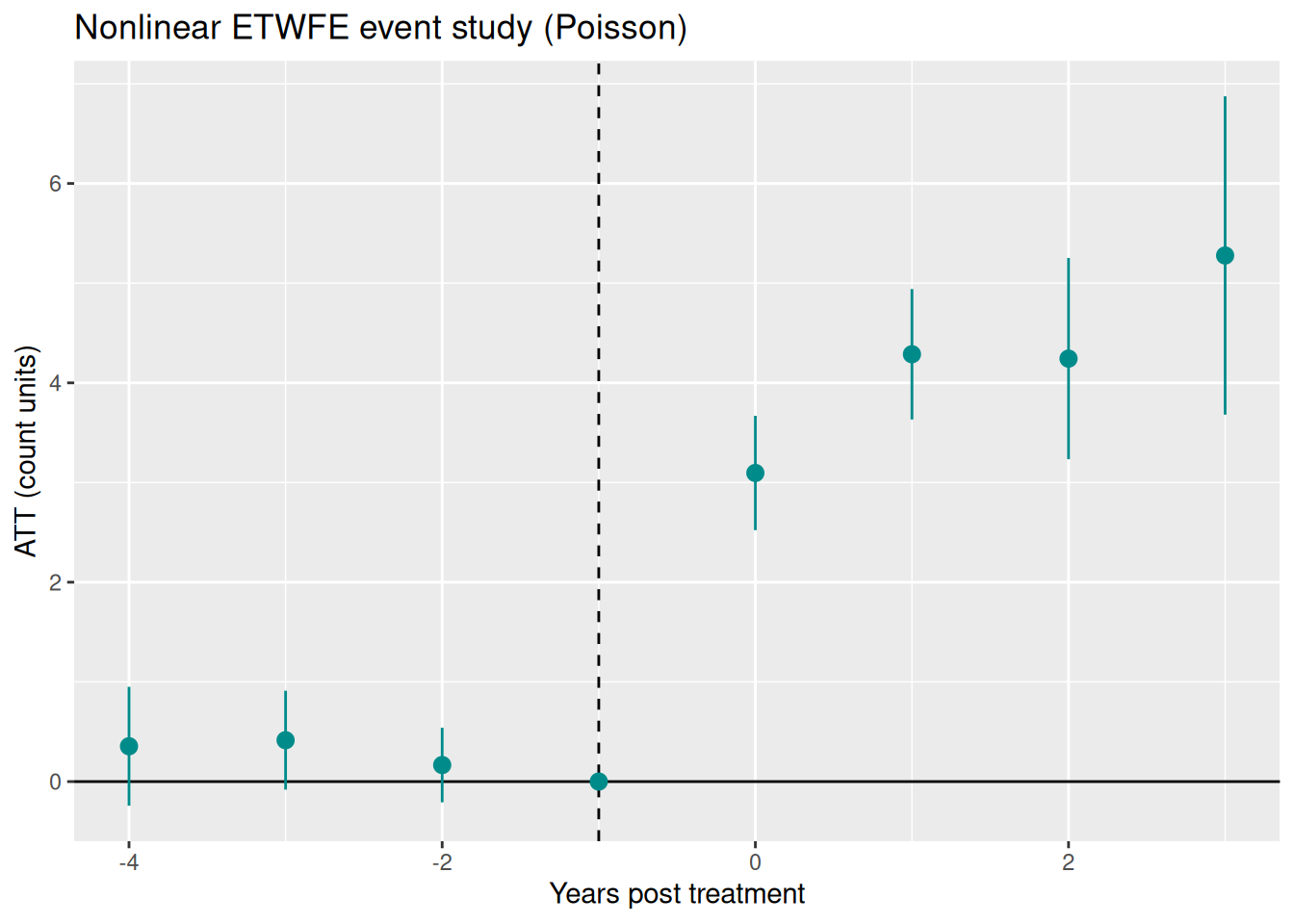
Pre-treatment estimates are close to zero, confirming parallel trends on the log scale holds in the simulation.
12.12.4 Comparison: linear ETWFE on log(count + 1)
A common alternative is to log-transform the count and run linear ETWFE. This is biased when zeros are present (the \(+1\) shift distorts the linear index) and misinterprets the scale of the effect. For comparison:
 .Dtreat Estimate Std. Error    z Pr(>|z|)     S 2.5 % 97.5 %
    TRUE     0.38     0.0319 11.9   <0.001 106.8 0.318  0.443

Term: .Dtreat
Type: response
Comparison: TRUE - FALSE
The linear model estimates the ATT on the \(\log(Y+1)\) scale — not the same quantity as the Poisson ATT and harder to interpret. When treatment effects are multiplicative, Poisson ETWFE is the more appropriate model.
12.13 Spatial Interference
Everything in this chapter so far assumes SUTVA: one unit’s outcome does not depend on another unit’s treatment. That is not always plausible. A treated municipality may affect deforestation in nearby untreated municipalities. A vaccinated household may reduce transmission to nearby households. A labor-market policy in one commuting zone may change flows to its neighbors. With this kind of spatial spillover, the usual DiD estimand no longer has the interpretation we want. Xu (2023) shows that ignoring interference can produce an estimand that is neither a direct effect nor a spillover effect.
Xu (2023, 2026) develops a doubly robust DiD that keeps the identifying logic of conditional parallel trends but adds an exposure mapping \(G_{it} = G(i, W_{-it})\) for unit \(i\)’s neighborhood treatment status. The estimand is the direct ATT at exposure level \(g\),
\[ \tau_g(t, c) = \frac{1}{|S_M|} \sum_{i \in S_M} \mathbb{E}[y_{it}(c, g) - y_{it}(\infty, g) \mid z_i, C_i = c, G_{it} = g], \]
where \(C_i\) is unit \(i\)’s first treatment period (so \(\{C_i > t\}\) is the not-yet-directly-treated comparison group), \(S_M = \{C_i = c\} \cup \{C_i > t\}\), and \(g\) is a chosen exposure level. The DR plug-in averages three pieces over \(S_M\): an IPW term from the treated cohort, an IPW term from the not-yet-treated, and a regression-imputation term, with three propensity models (\(\eta_{tc}\) for cohort, \(\eta_{tcg}\) and \(\eta_{t\infty g}\) for exposure) and two outcome-change regressions. It is consistent if either all three propensities or both outcome models are correctly specified.
The companion package didint implements this. The 2x2 base case (Xu 2023):
For staggered adoption (Xu 2026), did_int_staggered() loops over (cohort, time) cells with \(t \geq c\), restricts to \(S_M\) in each cell, fits the DR estimator, and aggregates across cells using joint-IF stacking (per-cell IFs share the never-treated comparison group, so independence-style SEs underestimate uncertainty noticeably). The vignettes/brazil_amazon.Rmd vignette of didint replicates Section III of Xu (2026), the Lista de Municípios Prioritários policy on Amazon deforestation, using the public Assunção-McMillan-Murphy-Souza-Rodrigues replication archive on Zenodo.
A Julia port with identical estimators is available as DidInterference.jl.
12.14 Persistent Outcomes and Heterogeneous Dynamics
Standard event-study TWFE regressions like
\[ Y_{it} = \alpha_i + \gamma_t + \sum_{j} D_{it}^j \delta_j + X_{it}'\beta + U_{it} \]
implicitly assume the residual has no serial dependence once unit and time fixed effects are absorbed. When outcomes are genuinely persistent — earnings, employment, consumption, anything with habits or adjustment costs — that assumption fails. The event-time dummies pick up the persistence on top of the true causal effect, producing spurious pre-trends and biased post-treatment estimates. With a true AR(1) DGP and persistence \(\rho_Y\), the omitted-variable bias on the event-time coefficients grows geometrically with the event-time horizon (Botosaru and Liu, 2025, Figure 1).
Botosaru and Liu (2025) introduce a dynamic panel with correlated random coefficients that handles both persistence and unit-level heterogeneity in dynamic responses:
\[ Y_{it} = \rho_Y Y_{i,t-1} + \alpha_i + \sum_j D_{it}^j \delta_{ij} + X_{it}'\beta + U_{it}, \]
with a parsimonious AR(1) structure on the event-time effects to keep dimensionality manageable:
\[ \delta_{ij} = \rho_\delta \delta_{i,j-1} + \varepsilon_{ij}, \quad j \geq 1. \]
The latent \(\lambda_i = (\alpha_i, \delta_{i0})\) is a unit-specific correlated random coefficient. A two-step semiparametric estimator: step 1 is quasi-maximum likelihood for the common parameters \((\rho_Y, \rho_\delta, \sigma_U^2, \sigma_\varepsilon^2, \beta)\) under a Gaussian working assumption on \(\lambda_i\) (consistent under misspecification of that working assumption); step 2 is Tweedie / Gaussian-conjugate empirical Bayes for the unit-level posterior trajectories \(\{\delta_{i,j}\}_{j=0}^J\), achieving asymptotic ratio optimality.
A companion paper (Botosaru and Liu 2026) adds a homogeneous-feedback extension: covariates \(X_{it}\) are allowed to adjust endogenously to past \(Y\) and treatment (the canonical example: minimum-wage policy affects wages directly and also indirectly through firms re-optimising input demand). Under the assumption that the covariate adjustment rule does not depend on \(\lambda_i\) given the observable history, the likelihood factors into a structural piece (for \(Y \mid X\), history) and a feedback piece (for \(X\) given history), each separately identified. The factorisation yields a clean decomposition of dynamic treatment effects into direct (through \(\delta_{i,j}\)) and indirect (through covariate feedback) components.
The package tvhte implements both papers:
library(tvhte)

# Fit on a panel with staggered cohorts and a covariate
fit <- tvhte(Y = panel_Y, Y0 = baseline_Y, t0 = cohort,
             J = max_event_time, X = panel_X)
print(fit)

# Feedback model + direct/indirect counterfactual decomposition
fb <- fit_feedback(panel_Y, baseline_Y, panel_X, baseline_X)
cf <- simulate_counterfactual(fit, fb, t0_star = alt_cohort)
A Julia port with the same API is at TVHTE.jl; both packages have deployed docs at https://xiangao.github.io/tvhte/ and https://xiangao.github.io/TVHTE.jl/.
12.15 Synthetic Control
The biggest problem with DiD is the PT assumption. There is not really a test for it, just like the unconfoundedness assumption. It is less demanding than unconfoundedness assumption, but nevertheless hard to justify sometimes.
Abadie (2010)’s idea is to construct a control unit, out of many control units (donor pool), which is a weighted average of all donor units, that then hopefully is very close to the treated unit in terms of outcome, in the pre-treatment periods. This works pretty well in practice, when you have a somewhat large donor pool. Of course there is still no test for post-treatment period, but for pre-treatment periods, usually it can get almost identical trend as the treated unit. This was designed for single treated unit at the beginning, but got extended to multiple treated units later on.
12.16 Synthetic DiD
Arkhangelsky et al (2021) tries to combine the idea of DiD and SC. SC assigns different weights to different control units. The standard DiD is a TWFE, assigning equal weights to all time periods and units.
To see that, DiD objective function:
\[ \small (\hat \tau^{did}, \hat \mu, \hat \alpha, \hat \beta) = \underset{\tau, \mu, \alpha, \beta}{argmin} { \Sigma_{i=1}^N \Sigma_{t=1}^T (Y_{it} - \mu - \alpha_i - \beta_t - W_{it} \tau)^2}\]
SC objective function: \[ (\hat \tau^{sc}, \hat \mu, \hat \beta) = \underset{\tau, \mu, \beta}{argmin} { \Sigma_{i=1}^N \Sigma_{t=1}^T \hat \omega_i^{sc} (Y_{it} - \mu - \beta_t - W_{it} \tau)^2}\]
It’s a unit-weighted regression with time effects. The weights are set to optimally match donor units to treated unit so that they are as close as possible, in each time point. Note there is no \(\alpha_i\), since it’s forced to be 0 — so SC is not simply DiD with weights: it also drops the unit fixed effects. The clean nesting is through SDiD below: DiD is SDiD with all unit and time weights set to 1, and SC is SDiD with the \(\alpha_i\) removed and time weights set to 1.
SDiD:
\[ \small (\hat \tau^{sdid}, \hat \mu, \hat \alpha, \hat \beta) = \underset{\tau, \mu, \alpha, \beta}{argmin} { \Sigma_{i=1}^N \Sigma_{t=1}^T \hat \omega_i^{sdid} \hat \lambda_t^{sdid} (Y_{it} - \mu - \alpha_i - \beta_t - W_{it} \tau)^2}\]
SDiD sets another weight in addition to SC weights, which changes over time. The SC weights are trying to construct a control unit that is close to the treated unit; the SDiD weights are trying to put more weights on pre-treatment periods that are more similar to post-treatment periods.
12.16.1 Example: California Proposition 99
library(synthdid)
data('california_prop99')
setup = panel.matrices(california_prop99)
tau.hat = synthdid_estimate(setup$Y, setup$N0, setup$T0)summary(tau.hat)$estimate
[1] -15.60383
$se
[,1]
[1,] NA
$controls
estimate 1
Nevada 0.124
New Hampshire 0.105
Connecticut 0.078
Delaware 0.070
Colorado 0.058
Illinois 0.053
Nebraska 0.048
Montana 0.045
Utah 0.042
New Mexico 0.041
Minnesota 0.039
Wisconsin 0.037
West Virginia 0.034
North Carolina 0.033
Idaho 0.031
Ohio 0.031
Maine 0.028
Iowa 0.026
$periods
estimate 1
1988 0.427
1986 0.366
1987 0.206
$dimensions
N1 N0 N0.effective T1 T0 T0.effective
1.000 38.000 16.388 12.000 19.000 2.783 tau.sc = sc_estimate(setup$Y, setup$N0, setup$T0)
tau.did = did_estimate(setup$Y, setup$N0, setup$T0)
estimates = list(tau.did, tau.sc, tau.hat)
names(estimates) = c('Diff-in-Diff', 'Synthetic Control', 'Synthetic Diff-in-Diff')
print(unlist(estimates)) Diff-in-Diff Synthetic Control Synthetic Diff-in-Diff
-27.34911 -19.61966 -15.60383 plot <- synthdid_plot(estimates, facet.vertical=FALSE,
control.name='control', treated.name='california',
lambda.comparable=TRUE, se.method = 'none',
trajectory.linetype = 1, line.width=.75, effect.curvature=-.4,
trajectory.alpha=.7, effect.alpha=.7,
diagram.alpha=1, onset.alpha=.7) +
theme(legend.position=c(.26,.07), legend.direction='horizontal',
legend.key=element_blank(), legend.background=element_blank(),
strip.background=element_blank(), strip.text.x = element_blank())plot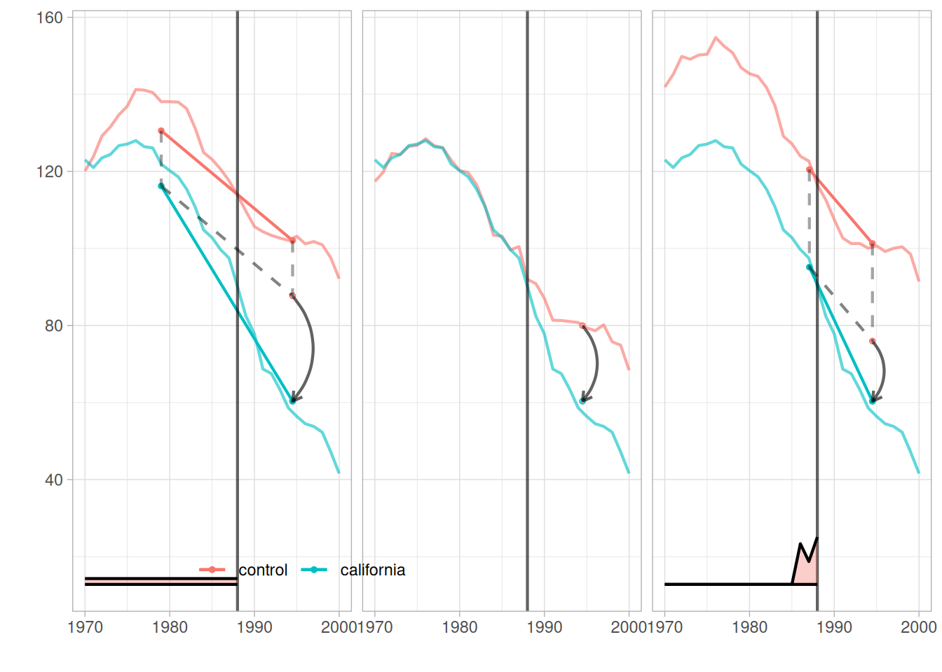
Note: \(\lambda_t\) is plotted at the bottom.