13  IV & Regression Discontinuity

If we have an unobserved confounder, unconfoundedness fails. Even when we have random experiment, we could have noncompliance. In that case, subjects are randomly assigned to treatment or control, but some of them do not comply with the assignment. In other words, there is selection bias in the sense that the treated group is self-selected. This selection could be correlated with the outcome.

13.1 Instrumental Variables

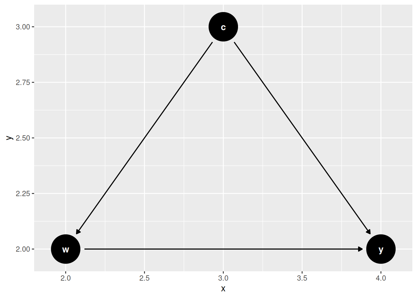
13.1.1 Uncontrolled Confounder

13.1.2 Why Does IV Work?

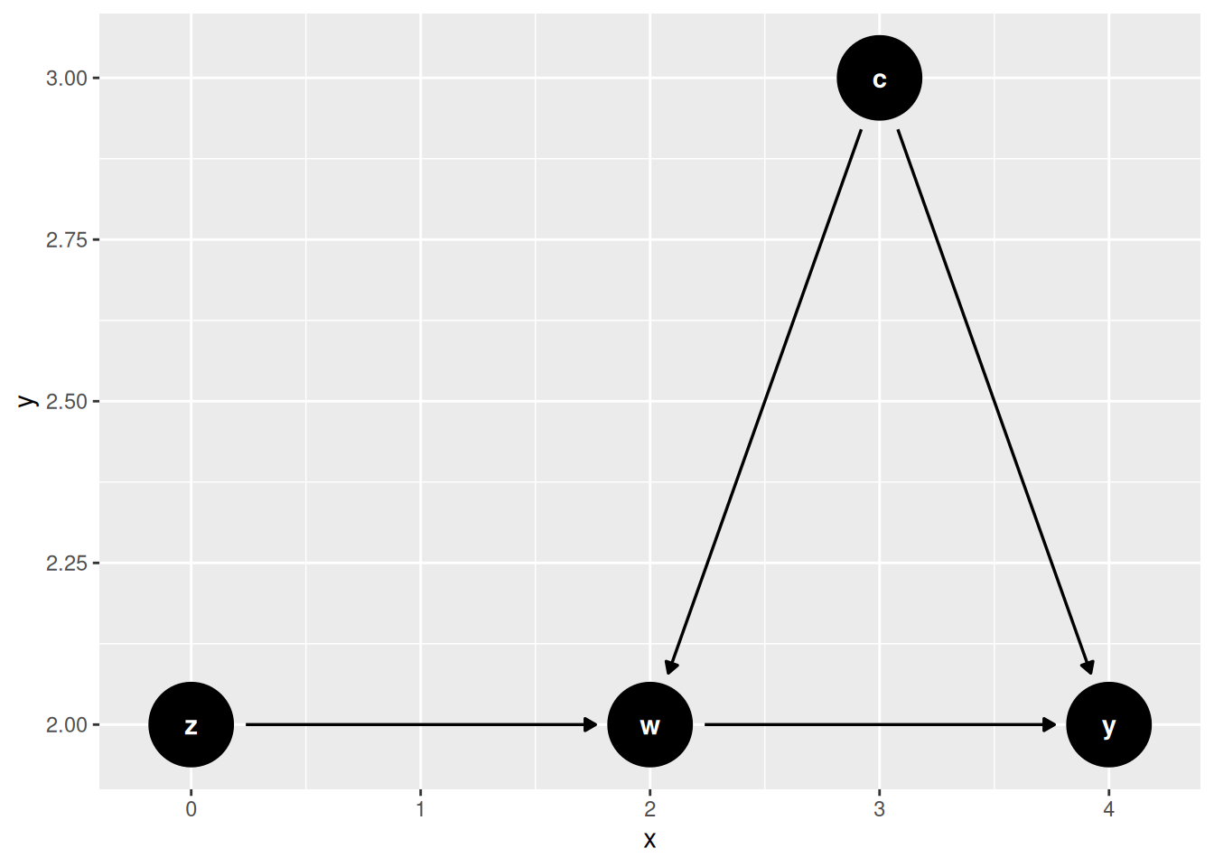
13.1.3 IV Under Potential Outcomes

• W has two potential outcomes W(1) and W(0), as a function of Z.
• Y has two potential outcomes Y(1) and Y(0), as a function of W.

Intention to Treat (ITT) is the average treatment effect of the treatment assignment Z. It is the difference between the average potential outcome under treatment and the average potential outcome under control. It is the average treatment effect of the treatment assignment Z, regardless of whether the subject complies with the assignment.

There are four possible groups of subjects in the case of binary treatment and binary instrument. For example treatment assignment Z and treated status W could be:

• Z=0, W=0: never-taker
• Z=0, W=1: complier
• Z=1, W=0: defier
• Z=1, W=1: always-taker

compliance groups

	W(1)=0	W(1)=1
W(0)=0	N	C
W(0)=1	D	A

These four groups (stratum) have different causal mechanisms. For example, the compliers are the only group that is affected by the treatment assignment Z in the same direction. The defiers are the only group that is affected by the treatment assignment Z in the opposite direction. The always-takers and never-takers are not affected by the treatment assignment Z.

Unfortunately we cannot identify the compliance group by looking at the data.

Z	W	G
0	0	C, N
0	1	A, D
1	0	N, D
1	1	C, A

13.1.4 Assumptions

• Exclusion restriction: \(Y(w, 1) = Y(w,0)\)
• Exogeneity of instrument: \(Z \perp [W(0),W(1), Y(0), Y(1)]\)
• Monotonicity (no defiers): \(W(0) \leq W(1)\)

13.1.5 LATE Identification

Since we excluded defiers, and the other two groups (always-takers and never-takers) are not affected by the treatment assignment Z. The only effect we can identify is the treatment effect on the compliers. This is called the Local Average Treatment Effect (LATE).

\[ \small \begin{aligned} & E[Y(Z=1) - Y(Z=0) | G = C] \\ &= \frac{E[Y(Z=1) - Y(Z=0)]}{P(W(1)=1, W(0)=0)} \\ &= \frac{E[Y|Z=1] - E[Y|Z=0]}{1-P(W=0|Z=1)-P(W=1|Z=0)} \text{ (rule out groups A and N) } \\ &= \frac{E[Y|Z=1] - E[Y|Z=0]}{P(W=1|Z=1)-P(W=1|Z=0)} \\ &= \frac{E[Y|Z=1] - E[Y|Z=0]}{E[W|Z=1)-E[W|Z=0]} \end{aligned} \]

13.1.6 Parametric Models

If we assume linearity, then this becomes the ratio of two OLS coefficients, sometimes called the Wald estimator.

\[ \begin{aligned} \tau_{ATE} &= \frac{E[Y|Z=1] - E[Y|Z=0]}{E[W|Z=1)-E[W|Z=0]} \\ &= \frac{Cov(Y,Z)}{Cov(W,Z)} \end{aligned} \]

Why do covariates help? Because we hope even if we don’t have exogeneity or exclusion assumption held, we would have those assumptions held within each level of \(X\).

13.1.7 Example

## DGP: data$y <- data$x + data$z + data$u
library(sem)
set.seed(66)
nobs=10000
nDim = 3
sdww = 1
sdzz=1
sdmm=1
## here we have three variables x,z,w.
## m is the omitted variable,x and m are correlated,  z is the instrument, which is correlated with x, but not m.  u is indepent of everything else.
crwm=.6
crmz=0
crwz=.8
covarMat = matrix( c(sdww^2, crwm^2, crwz^2, crwm^2, sdmm^2, crmz^2,  crwz^2, crmz^2, sdzz^2 ) , nrow=nDim , ncol=nDim )
data  = data.frame(MASS::mvrnorm(n=nobs, mu=rep(0,nDim), Sigma=covarMat ))
names(data) <- c('w','m','z')
data$u <- rnorm(nobs,0,1)
# dgp
data$y <- data$w +  data$m + data$u
lm <- lm(y~w, data=data)
lm.full <- lm(y~ w + m, data=data)
tsls.model <- sem::tsls(y ~ w , ~ z , data=data)

# lm is biased
summary(lm)$coefficients

                Estimate Std. Error    t value  Pr(>|t|)
(Intercept) -0.003580657 0.01372253 -0.2609326 0.7941498
w            1.358930425 0.01396918 97.2805995 0.0000000

# lm.full is good
summary(lm.full)$coefficients

               Estimate  Std. Error    t value  Pr(>|t|)
(Intercept) 0.001833551 0.009973474  0.1838428 0.8541405
w           0.992438925 0.010868032 91.3172630 0.0000000
m           1.013403057 0.010723435 94.5035837 0.0000000

# tsls is good.
summary(tsls.model)$coefficients

               Estimate Std. Error    t value  Pr(>|t|)
(Intercept) 0.006008287 0.01424525  0.4217749 0.6731984
w           0.972416527 0.02312558 42.0493890 0.0000000

13.1.8 Control Function Approach

Two-stage least squares can be implemented equivalently via the control function (CF) approach. Understanding why makes the extension to nonlinear models (next chapter) transparent.

Algebraic motivation. Because w is endogenous, decompose the structural error:

\[\varepsilon = \rho v + \eta, \qquad v \equiv w - E[w \mid z], \qquad E(z\eta) = 0,\; E(zv) = 0.\]

If we knew \(v\), controlling for it directly would eliminate the confounding channel. We don’t know \(v\), but the first-stage residual \(\hat v = w - \hat w\) is a consistent estimate. Substituting into the structural equation:

\[y = \alpha + \beta w + \rho\,\hat v + \text{error}.\]

OLS on this augmented second stage gives a consistent \(\hat\beta\) — identical to 2SLS by the Frisch–Waugh–Lovell (FWL) theorem. The coefficient \(\hat\rho\) on \(\hat v\) doubles as a Durbin–Wu–Hausman (DWH) endogeneity test: under \(H_0\) (w is exogenous), \(\rho = 0\).

# Manual 2SLS, explicitly
stage1     <- lm(w ~ z, data = data)
data$w_hat <- fitted(stage1)
tsls_manual <- lm(y ~ w_hat, data = data)

# Control function: first-stage residual v_hat in the augmented regression
data$v_hat <- residuals(stage1)
lm_cf      <- lm(y ~ w + v_hat, data = data)

# Compare β̂_w from manual 2SLS and CF — should be identical by FWL
coef_tsls <- coef(tsls_manual)["w_hat"]
coef_cf   <- coef(lm_cf)["w"]
sprintf("Manual 2SLS   beta_w = %.8f", coef_tsls)

[1] "Manual 2SLS   beta_w = 0.97241653"

sprintf("Control funct beta_w = %.8f", coef_cf)

[1] "Control funct beta_w = 0.97241653"

# DWH endogeneity test: t-stat on v_hat
rho_summary <- summary(lm_cf)$coefficients["v_hat", ]
sprintf("DWH test on v_hat: coef = %.4f  se = %.4f  t = %.3f  p = %.4g",
        rho_summary["Estimate"], rho_summary["Std. Error"],
        rho_summary["t value"], rho_summary["Pr(>|t|)"])

[1] "DWH test on v_hat: coef = 0.6366  se = 0.0279  t = 22.827  p = 1.797e-112"

The two \(\hat\beta_w\) values agree to machine precision, confirming FWL. The large \(|t|\) on \(\hat v\) rejects \(H_0\!:\rho = 0\), confirming that w is endogenous.

Why FWL fails in nonlinear models. FWL relies on the residual-maker matrix being idempotent and the second stage being linear — both fail once we replace OLS with Poisson or Probit. In a nonlinear second stage, \(\hat v\) must enter inside the link function (e.g. \(\exp(\mathbf{x}\boldsymbol\beta + \rho \hat v)\)), which requires a structural assumption beyond instrument exogeneity. This is the subject of the next chapter.

13.2 Regression Discontinuity Design

RDD (regression discontinuity design) is a quasi-experimental design that is used to estimate causal effects of interventions when assignment to the intervention is determined by whether a subject’s value on an observed covariate exceeds a threshold. The idea is that the assignment is as good as random, so we can estimate the causal effect of the intervention by comparing the outcomes of subjects who are just above and just below the threshold.

13.2.1 Sharp RDD

We have a continuous variable \(X\), called the running variable, which determines the binary treatment \(W\). The treatment is assigned according to a threshold \(c\). The outcome variable \(Y\) is a function of \(X\) and \(W\).

\[ W=\mathbb{1}(X>c)\]

Lee (2008) studies the effect of incumbency advantage in elections. His identification strategy is based on the discontinuity generated by the rule that the party with a majority vote share wins. The forcing variable \(X_i\) is the difference in vote share between the Democratic and Republican parties in one election, with the threshold \(c = 0\). The outcome variable \(Y_i\) is vote share at the second election.

library(rdrobust)
data(rdrobust_RDsenate)
rdplot(x=rdrobust_RDsenate$margin, y=rdrobust_RDsenate$vote)

13.2.2 Identification of SRDD

\[ \tau_{RD} = \lim_{x \to c^+} E[Y|X=x] - \lim_{x \to c^-} E[Y|X=x] \]

In words, the treatment effect is the difference in the outcome from the right side and from the left side. This is the same as the difference in the outcome at the threshold, as if the treatment is assigned randomly.

13.2.3 Estimation of SRDD

GPA <- runif(1000, 0, 4)
future_success <- 10 + 1.5 * GPA + 2 * (GPA <= 3) + rnorm(1000)
rdplot(x=GPA, y=future_success, c=3)

# estimate the sharp RDD model
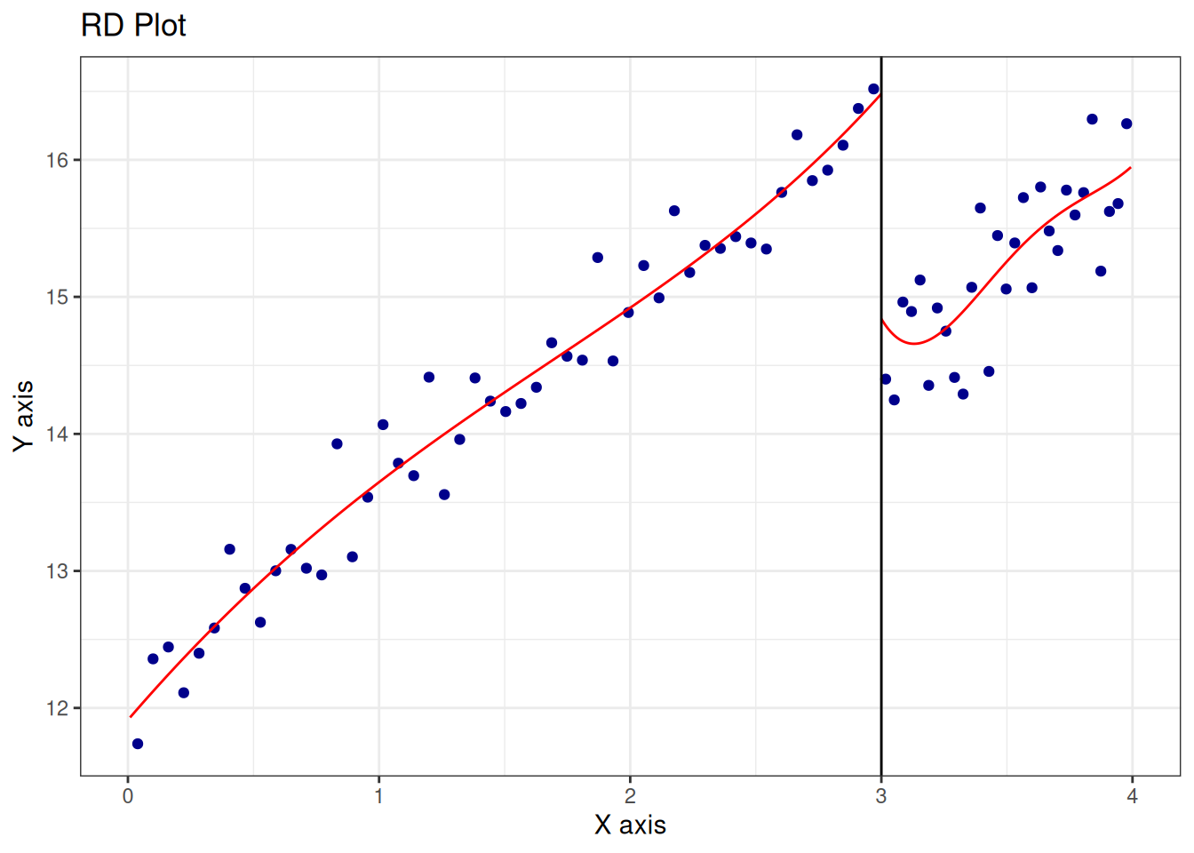
rdd_gpa <- rdrobust(x=GPA, y=future_success, c=3)
summary(rdd_gpa)

Sharp RD estimates using local polynomial regression.

Number of Obs.                 1000
BW type                       mserd
Kernel                   Triangular
VCE method                       NN

Number of Obs.                  745          255
Eff. Number of Obs.              71           71
Order est. (p)                    1            1
Order bias  (q)                   2            2
BW est. (h)                   0.322        0.322
BW bias (b)                   0.525        0.525
rho (h/b)                     0.613        0.613
Unique Obs.                     745          255

=====================================================================
                   Point    Robust Inference
                Estimate         z     P>|z|      [ 95% C.I. ]       
---------------------------------------------------------------------
     RD Effect    -1.859    -4.562     0.000    [-2.607 , -1.040]    
=====================================================================

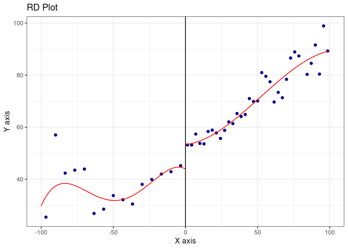
13.2.4 Nonparametric Estimation

rdd_house <- rdrobust(x=rdrobust_RDsenate$margin, y=rdrobust_RDsenate$vote, c=0, all=TRUE)
summary(rdd_house)

Sharp RD estimates using local polynomial regression.

Number of Obs.                 1297
BW type                       mserd
Kernel                   Triangular
VCE method                       NN

Number of Obs.                  595          702
Eff. Number of Obs.             360          323
Order est. (p)                    1            1
Order bias  (q)                   2            2
BW est. (h)                  17.754       17.754
BW bias (b)                  28.028       28.028
rho (h/b)                     0.633        0.633
Unique Obs.                     595          665

=======================================================================================
        Method     Coef. Std. Err.         z     P>|z|      [ 95% C.I. ]       
=======================================================================================
  Conventional     7.414     1.459     5.083     0.000     [4.555 , 10.273]    
Bias-Corrected     7.507     1.459     5.146     0.000     [4.647 , 10.366]    
        Robust     7.507     1.741     4.311     0.000     [4.094 , 10.919]    
=======================================================================================

13.2.5 Fuzzy RDD

In fuzzy RDD, the treatment is assigned according to a threshold \(c\), but there exist non-compliance. This is similar to IV case.

\[ \tau_{FRD} = \frac{\lim_{x \to c^+} E[Y|X=x] - \lim_{x \to c^-} E[Y|X=x]}{\lim_{x \to c^+} E[W|X=x] - \lim_{x \to c^-} E[W|X=x]} \]

For example, if food stamp eligibility is given to all households below a certain income, but not all households receive the food stamps. In other words, income does not solely determine the assignment. Cutoff point increases the probability of treatment but doesn’t completely determine treatment.

FRDD is IV.

13.2.6 FRDD Example

Fetter (2013)’s main question of interest is how much of the increase in the home ownership rate in the midcentury US was due to mortgage subsidies given out by the government.

We’re using the running variable quarter of birth (qob), which has been centered on the quarter of birth you’d need to be to be eligible for a mortgage subsidy for fighting in the Korean War (qob_minus_kw). This determines whether you were a veteran of either the Korean War or World War II (vet_wwko).

vet <- causaldata::mortgages
# Create an "above-cutoff" variable as the instrument
vet <- vet %>% mutate(above = qob_minus_kw > 0)
# Impose a bandwidth of 12 quarters on either side
vet <- vet %>%  filter(abs(qob_minus_kw) < 12)
m <- feols(home_ownership ~
    nonwhite  | # Control for race
    bpl + qob | # fixed effect controls
    qob_minus_kw*vet_wwko ~ # Instrument our standard RDD
    qob_minus_kw*above, # with being above the cutoff
    se = 'hetero', # heteroskedasticity-robust SEs
    data = vet)
summary(m)

TSLS estimation - Dep. Var.: home_ownership
                  Endo.    : qob_minus_kw, vet_wwko,
                  qob_minus_kw:vet_wwko
                  Instr.   : qob_minus_kw, above, qob_minus_kw:above
Second stage: Dep. Var.: home_ownership
Observations: 56,901
Fixed-effects: bpl: 52,  qob: 4
Standard-errors: Heteroskedasticity-robust 
                           Estimate Std. Error   t value   Pr(>|t|)    
fit_qob_minus_kw          -0.007151   0.001773  -4.03209 5.5355e-05 ***
fit_vet_wwko               0.170172   0.045933   3.70479 2.1177e-04 ***
fit_qob_minus_kw:vet_wwko -0.002853   0.002637  -1.08159 2.7944e-01    
nonwhite                  -0.190434   0.006892 -27.63141  < 2.2e-16 ***
---
Signif. codes:  0 '***' 0.001 '**' 0.01 '*' 0.05 '.' 0.1 ' ' 1
RMSE: 0.441909     Adj. R2: 0.066481
                 Within R2: 0.051235
F-test (1st stage), qob_minus_kw         : stat = 14,276,113,954,118,300,000,000,000,000,000,000.0000, p < 2.2e-16 , on 3 and 56,842 DoF.
F-test (1st stage), vet_wwko             : stat =                                          2,541.2120, p < 2.2e-16 , on 3 and 56,842 DoF.
F-test (1st stage), qob_minus_kw:vet_wwko: stat =                                         14,465.7762, p < 2.2e-16 , on 3 and 56,842 DoF.
                               Wu-Hausman: stat =                                              4.4989, p = 0.003679, on 3 and 56,839 DoF.

controls <- vet %>%
    select(nonwhite, bpl, qob) %>%
    mutate(qob = factor(qob))
conmatrix <- model.matrix(~., data = controls)
m <- rdrobust(vet$home_ownership,
              vet$qob_minus_kw,
              fuzzy = vet$vet_wwko,
              c = 0,
              covs = conmatrix)
m$Estimate

        tau.us    tau.bc       se.us       se.rb
[1,] 0.8339441 0.8320108 0.002823468 0.003482787

These two results are very different, which is one of RDD’s problems. It can be sensitive to model selection. For example, in the case of 2SLS, it’s a linear model. In the case of “rdrobust”, it’s a local regression, which can be sensitive to bandwidth selection.