# Shift-Share Instrumental Variables
```{r}
#| include: false
library(tidyverse)
library(fixest)
library(ggplot2)
library(knitr)
```
Shift-share, or Bartik, instruments combine local industry shares with
industry-level shocks. The idea is simple: a location with a large baseline
share in an industry is more exposed to shocks in that industry. The
difficult part is not constructing the instrument. The difficult part is
stating what is assumed exogenous: the shares, the shocks, or both.
## The construction
For each location $\ell$ and industry $k$, let $s_{\ell k}$ be the share of
local employment in industry $k$ at baseline, and let $g_k$ be a national
growth rate (or trade shock) for that industry. The shift-share instrument is
$$
B_\ell \;=\; \sum_{k=1}^{K} s_{\ell k}\, g_k.
$$
This is "shift-share" because it combines a local share with an
industry-level shift. @bartik-1991 used local industry mix to predict local
employment growth. @autor-dorn-hanson-2013 used local industry shares
interacted with industry-level Chinese import growth in other high-income
countries.
The first-stage regression is then
$$
\Delta L_\ell \;=\; \pi_0 + \pi_1 B_\ell + X_\ell'\gamma + \epsilon_\ell,
$$
with $B_\ell$ instrumenting for the observed local shock in a 2SLS for the
outcome of interest.
## Two identification views
There are two ways to justify a shift-share instrument. They put the
exogeneity assumption on different objects.
### Share view (GPSS 2020)
Treat the shares $s_{\ell k}$ as the source of identifying variation, with the
shocks $g_k$ acting as weights. The instrument is valid if shares are
exogenous to the outcome (conditional on controls).
@goldsmith-pinkham-sorkin-swift-2020 (henceforth GPSS) prove that the
shift-share IV is numerically equivalent to a GMM combination of $K$
just-identified IVs, one per industry share:
$$
\hat\beta^{SS} \;=\; \sum_{k=1}^{K} \hat\alpha_k\, \hat\beta_k,
$$
where $\hat\beta_k$ is the just-identified IV using share $s_{\cdot k}$ alone
and $\hat\alpha_k$ is the **Rotemberg weight**. This gives an important
diagnostic: which industry shares are driving the estimate?
### Shock view (BHJ 2022)
Treat the shocks $g_k$ as the source of identifying variation. Shares are
exposure weights. Under this view, shocks should be uncorrelated with the
second-stage unobservables, conditional on industry-level controls.
@borusyak-hull-jaravel-2022 (henceforth BHJ) show how to rewrite the
regression at the shock level.
The two views are not mutually exclusive. In an application, we should be
clear which one is being defended and report diagnostics for both.
## Inference
Standard OLS or cluster-robust standard errors on the regional regression
**underestimate uncertainty** because the same industry shocks appear in many
regions, inducing cross-region correlation that region-level clustering does
not capture. Two corrections are now standard:
- **Cluster on shocks (BHJ)**: equivalent to running the regression at the
industry-shock level. Implemented via shock-level reweighting.
- **AKM SE** [@adao-kolesar-morales-2019]: explicit formula for SE accounting
for shock-level correlation. Available in the `ShiftShareSE` R package.
## Simulation: build intuition
Use a small DGP with regions, industries, and a known causal effect.
```{r}
#| label: sim-data
#| cache: true
n_region   <- 500
n_industry <- 20
beta_true  <- 0.5

df     <- read_csv("data/shift_share_sim.csv", show_col_types = FALSE)
shares <- as.matrix(read_csv("data/shift_share_shares.csv", show_col_types = FALSE))
# This simulation is constructed to satisfy the Borusyak et al. (2022)
# shock-exogeneity assumption: the industry-level shocks are drawn
# independently of the region-level confounder `u` and of the shares
# themselves. The shares are allowed to be endogenous (correlated with
# region characteristics) -- it is specifically the shocks that must be
# "as good as randomly assigned" for this identification argument, which is
# a different (and in this simulation, the maintained) assumption from the
# Goldsmith-Pinkham et al. (2020) shares-exogeneity view discussed above.
shocks <- read_csv("data/shift_share_shocks.csv", show_col_types = FALSE)$shock
u      <- df$u
head(df)
```
A naive OLS suffers from the confounder `u`:
```{r}
#| label: naive-ols
#| cache: true
ols  <- feols(Y ~ X, data = df)
ivss <- feols(Y ~ 1 | X ~ B, data = df)
etable(ols, ivss, headers = c("OLS", "Shift-share IV"),
       digits = 3, digits.stats = 3, fitstat = ~ . + ivf)
```
OLS is biased upward by the confounder; the shift-share IV recovers a
value close to the true effect of `r beta_true`. With concentrated industry
shares and 20 industries, the first-stage F is well above 100.
### Rotemberg weights
The GPSS decomposition says the shift-share IV is a weighted average of
$K$ just-identified IVs (one per industry share). Compute the weights:
```{r}
#| label: rotemberg
#| cache: true
# Rotemberg weight for industry k (using centered moments to match the
# demeaned 2SLS regression):
#   alpha_k = g_k * Cov(s_{.k}, X) / sum_j g_j * Cov(s_{.j}, X)
# Each industry's just-identified IV estimate uses s_{.k} as instrument:
#   beta_k = Cov(s_{.k}, Y) / Cov(s_{.k}, X)
# GPSS prove the shift-share IV estimate equals sum_k alpha_k * beta_k.

cov_sk_X <- sapply(1:n_industry, function(k) cov(shares[, k], df$X))
cov_sk_Y <- sapply(1:n_industry, function(k) cov(shares[, k], df$Y))
denom    <- sum(shocks * cov_sk_X)

alpha  <- shocks * cov_sk_X / denom
beta_k <- cov_sk_Y / cov_sk_X

rotemberg <- tibble(industry = 1:n_industry,
                    shock    = shocks,
                    weight   = alpha,
                    beta_k   = beta_k)

kable(rotemberg, digits = 3,
      caption = paste0("Rotemberg decomposition. Sum of alpha*beta_k = ",
                       round(sum(alpha * beta_k), 3),
                       " (= shift-share IV estimate of ",
                       round(coef(ivss)["fit_X"], 3), ")."))
```
Two diagnostics matter:
1. **Weight concentration**: if one or two industries carry most of the
weight, the identifying variation is essentially coming from those
industries' shares. Their exogeneity is the assumption you're really
leaning on.
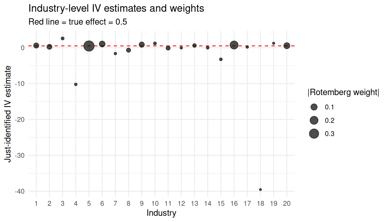
2. **Heterogeneous $\hat\beta_k$**: in this benign simulation, the
industry-specific IVs are all near the true effect (with sampling noise).
In real data, if a few industries give wildly different estimates, the
"average" shift-share IV is averaging over heterogeneous treatment effects
you should report explicitly.
```{r}
#| label: rotemberg-plot
#| cache: true
#| fig-height: 4
#| fig-width: 7
ggplot(rotemberg, aes(x = factor(industry), y = beta_k, size = abs(weight))) +
  geom_hline(yintercept = beta_true, linetype = "dashed", color = "red") +
  geom_point(alpha = 0.7) +
  scale_size_continuous(name = "|Rotemberg weight|") +
  labs(x = "Industry", y = "Just-identified IV estimate",
       title = "Industry-level IV estimates and weights",
       subtitle = paste("Red line = true effect =", beta_true)) +
  theme_minimal()
```
### What goes wrong when shares are endogenous
Now break the share-exogeneity assumption: make industry 1's share correlated
with the second-stage error.
```{r}
#| label: bad-shares
#| cache: true
# Re-do shares so industry 1's share covaries with a new confounder v
v <- read_csv("data/shift_share_bad_v.csv", show_col_types = FALSE)$v
shares_bad <- shares
shares_bad[, 1] <- pmax(0.01, shares[, 1] + 0.15 * v)
shares_bad <- shares_bad / rowSums(shares_bad)   # renormalise to sum to 1

bad_noise <- read_csv("data/shift_share_bad_noise.csv", show_col_types = FALSE)
B_bad <- as.numeric(shares_bad %*% shocks)
X_bad <- B_bad + 0.3 * u + bad_noise$noise_x
Y_bad <- beta_true * X_bad + u + 0.6 * v + bad_noise$noise_y

df_bad <- tibble(X = X_bad, Y = Y_bad, B = B_bad)
ivss_bad <- feols(Y ~ 1 | X ~ B, data = df_bad)
cat("True beta:", beta_true, "\n")
cat("Shift-share IV with bad share 1:", round(coef(ivss_bad)["fit_X"], 3), "\n")
# Rotemberg weights recomputed under the bad shares
cov_sk_X_bad <- sapply(1:n_industry, function(k) cov(shares_bad[, k], X_bad))
alpha_bad    <- shocks * cov_sk_X_bad / sum(shocks * cov_sk_X_bad)
cat("Rotemberg weight of industry 1:", round(alpha_bad[1], 3),
    "-- rank", rank(-abs(alpha_bad))[1], "of", n_industry, "\n")
# Leave-one-industry-out: rebuild the instrument without industry 1
B_loo    <- as.numeric(shares_bad[, -1] %*% shocks[-1])
ivss_loo <- feols(Y ~ 1 | X ~ B, data = tibble(X = X_bad, Y = Y_bad, B = B_loo))
cat("Shift-share IV without industry 1:", round(coef(ivss_loo)["fit_X"], 3), "\n")
```
The estimate is biased, and the bias comes from one industry's share being
related to the error. Note which diagnostic catches it. Rotemberg weights
measure *influence* --- whose exogeneity the estimate leans on --- not
endogeneity: the offending industry carries a weight of only 0.11, third
largest of twenty, yet it alone moves the estimate from 0.5 to 0.8. The
leave-one-industry-out check is what isolates it: rebuilding the instrument
without industry 1 restores the estimate to 0.48.
## Empirical: the China shock (Autor, Dorn, Hanson 2013)
The standard shift-share application is the China-shock study of
@autor-dorn-hanson-2013 (henceforth ADH). Commuting zones are exposed
differently to Chinese import competition because their baseline industry
mixes differ. The instrument is
$$
\text{IV}_\ell \;=\; \sum_k \frac{L_{\ell k,\,1990}}{L_{\ell,\,1990}}\,
\frac{\Delta M^{other}_{k}}{L_{k,\,1990}},
$$
where the shocks $\Delta M^{other}_k$ are growth in Chinese imports into
other high-income countries. This leave-one-out construction removes
US-specific demand from the shock. In the actual ADH design the employment
shares are lagged one census behind the outcome period (e.g. 1980 employment
for the 1990--2000 stack), precisely to mitigate share endogeneity; we date
everything to 1990 here to keep the notation light.
```{r}
#| label: adh-skeleton
#| eval: false
#| echo: true
# David Dorn distributes the replication data at
# https://www.ddorn.net/data.htm — files needed:
#   workfile_china.dta  (commuting zone data, 1990-2007)
#   industry_shares.csv (czone-industry shares)
#   industry_imports.csv (industry-level imports)

library(haven)
library(fixest)

cz   <- read_dta("workfile_china.dta")
fit  <- feols(d_sh_empl_mfg ~ 1 | d_tradeusch_pw ~ d_tradeotch_pw_lag,
              data = cz,
              cluster = ~ statefip)
summary(fit)
```
Modern best-practice extensions of the basic ADH regression. These blocks are
schematic --- they do not run here, so check argument names against the
current package documentation before adapting them:
```{r}
#| label: adh-modern
#| eval: false
#| echo: true
# 1. Rotemberg weights via the bartik.weight package (Goldsmith-Pinkham)
# devtools::install_github("paulgp/bartik-weight")
library(bartik.weight)
rw <- bw(cz, master = master_spec, y = "d_sh_empl_mfg",
         x = "d_tradeusch_pw", weight = "timepwt48",
         G = G_growth, Z = Z_shares)

# Plot the Rotemberg weights to see which industries drive the estimate
plot(rw)

# 2. Adão-Kolesár-Morales standard errors
# devtools::install_github("kolesarm/ShiftShareSE")
library(ShiftShareSE)
ivreg_ss(d_sh_empl_mfg ~ d_tradeusch_pw + controls,
         X = "d_tradeotch_pw_lag",
         data = cz, W = shock_weights, region_cvar = "czone",
         method = "akm0")

# 3. BHJ shock-level inference: collapse to shock (industry-period) level
# devtools::install_github("borusyak/shift-share")
library(ssaggregate)
shocks_data <- ssaggregate(data = cz, vars = c("d_sh_empl_mfg",
                                                "d_tradeusch_pw"),
                            shock = "d_tradeotch_pw_lag", weights = "timepwt48",
                            l = "czone", n = "industry", t = "year",
                            s = "share")
# Now regress at shock level — interpretation: shock-level IV
feols(d_sh_empl_mfg ~ 1 | d_tradeusch_pw ~ shock, data = shocks_data)
```
For a new shift-share paper, I would expect Rotemberg weights, AKM standard
errors, and a BHJ shock-level version or an explanation for why it is not
appropriate.
## Summary
- Shift-share IV combines local shares and industry shocks.
- The GPSS view puts exogeneity on shares; the BHJ view puts it on shocks.
- Rotemberg weights show which industry shares drive the 2SLS estimate.
- Region-level clustering is usually too optimistic. Use AKM standard errors
or shock-level inference when possible.
- In R, `fixest`, `bartik.weight`, `ShiftShareSE`, and `ssaggregate` cover
most of the workflow.