16  G-Methods for Time-Varying Treatments

library(tidyverse)
library(ltmle)
library(ipw)
library(survey)
library(broom)

Most chapters so far use one treatment decision. Many real problems are longitudinal. A patient receives medication at several visits. A worker can enter training in more than one year. Treatment changes over time, and covariates respond to past treatment. Those covariates then affect future treatment. Standard regression adjustment can fail in this setting.

Related reading: The g-estimation with time-varying covariates chapter of Topics on Econometrics and Causal Inference derives the identification result with sequential ignorability and applies the parametric g-formula to a worked binary-treatment example. The LMTP framework (for continuous and modified-policy interventions) is covered in Longitudinal modified treatment policy (LMTP) and in the Continuous Treatments chapter.

The main tools are:

1. G-formula: simulate outcomes under a treatment regime.
2. IPTW: reweight observations by the probability of their treatment history.
3. Marginal structural models: fit a treatment-history regression in the weighted population.
4. Longitudinal TMLE: combine outcome and treatment-history models.

16.1 The time-varying confounding problem

The methods in this chapter are Robins’s g-methods. The g-formula is Robins (1986); marginal structural models and IPTW are Robins, Hernán and Brumback (2000); Hernán and Robins (2020) is the standard reference for the whole family.

Consider a two-period example:

• \(L_0\): baseline covariate (e.g. health status at study entry)
• \(A_0\): treatment at time 0 (e.g. medication)
• \(L_1\): covariate at time 1, influenced by \(A_0\) (e.g. health status after first dose)
• \(A_1\): treatment at time 1, influenced by \(L_1\)
• \(Y\): outcome at the end of follow-up (e.g. mortality)

The DAG:

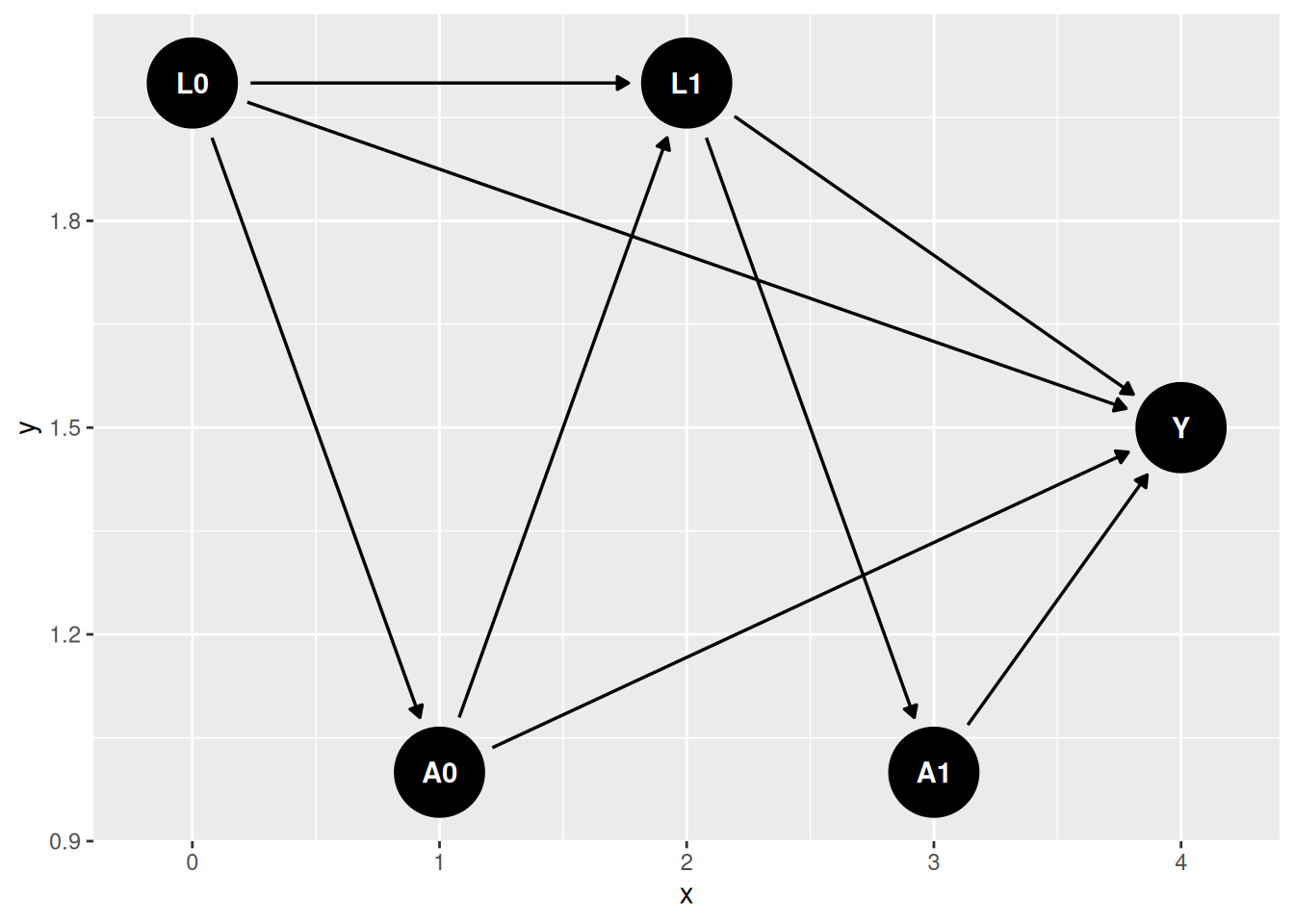
\(L_1\) is the problem variable. It confounds the effect of \(A_1\) on \(Y\), so we would like to adjust for it. But it is also affected by \(A_0\), so adjusting for it blocks part of the effect of \(A_0\). Regression without \(L_1\) is confounded; regression with \(L_1\) over-controls.

16.1.1 Simulating the failure of regression

We simulate \(n = 5000\) units over two periods. The baseline covariate is \(L_0 \sim N(0,1)\), and the first treatment is \(A_0 \sim \text{Bernoulli}(\Lambda(-0.5 + 0.8L_0))\). The time-varying confounder responds to the first treatment, \(L_1 = 0.5L_0 + 1.0A_0 + \nu\) with \(\nu \sim N(0,1)\), and the second treatment responds to it, \(A_1 \sim \text{Bernoulli}(\Lambda(-0.5 + 0.8L_1))\). The outcome is \(Y = 0.5A_0 + 0.5A_1 + 0.5L_1 + 0.5L_0 + \varepsilon\) with \(\varepsilon \sim N(0,1)\).

The truth follows from the coefficients. \(A_1\) has a total effect of 0.5. \(A_0\) has a direct effect of 0.5 plus an indirect effect through \(L_1\) of \(1.0 \times 0.5 = 0.5\), so its total effect is 1.0. Always treating versus never treating is therefore worth \(1.0 + 0.5 = 1.5\).

We fit two regressions that a reader might reach for first: one omitting \(L_1\) and one including it.

set.seed(1)
n <- 5000

# Baseline covariate
L0 <- rnorm(n)
# Treatment at t=0 depends on L0
A0 <- rbinom(n, 1, plogis(-0.5 + 0.8 * L0))
# Time-varying confounder L1: affected by A0 (and L0)
L1 <- 0.5 * L0 + 1.0 * A0 + rnorm(n)
# Treatment at t=1 depends on L1
A1 <- rbinom(n, 1, plogis(-0.5 + 0.8 * L1))
# Outcome: each treatment has a direct effect of 0.5 on Y.
# A0 ALSO affects Y indirectly through L1 (A0 -> L1 -> Y): the L1 path
# contributes 1.0 * 0.5 = 0.5, so A0's TOTAL effect is 0.5 + 0.5 = 1.0,
# while A1's total effect is 0.5. Always-vs-never total effect = 1.5.
Y <- 0.5 * A0 + 0.5 * A1 + 0.5 * L1 + 0.5 * L0 + rnorm(n)

df <- tibble(L0, A0, L1, A1, Y)

cat("True total effect of always-treated vs never-treated: 1.5\n\n")

True total effect of always-treated vs never-treated: 1.5

# Naive regression 1: ignore L1
naive_no_L1 <- lm(Y ~ A0 + A1 + L0, data = df)
cat(sprintf("Naive (no L1): A0=%.3f, A1=%.3f, total=%.3f\n",
            coef(naive_no_L1)["A0"], coef(naive_no_L1)["A1"],
            coef(naive_no_L1)["A0"] + coef(naive_no_L1)["A1"]))

Naive (no L1): A0=0.979, A1=0.834, total=1.813

# Naive regression 2: include L1
naive_with_L1 <- lm(Y ~ A0 + A1 + L0 + L1, data = df)
cat(sprintf("Naive (with L1): A0=%.3f, A1=%.3f, total=%.3f\n",
            coef(naive_with_L1)["A0"], coef(naive_with_L1)["A1"],
            coef(naive_with_L1)["A0"] + coef(naive_with_L1)["A1"]))

Naive (with L1): A0=0.545, A1=0.503, total=1.048

Neither regression recovers the true total effect of 1.5. Omitting \(L_1\) gives 1.813, too high; including it gives 1.048, too low. The truth is between them, and no choice between these two specifications reaches it.

The two failures have different sources:

• Excluding \(L_1\) leaves confounding from \(L_1 \to A_1\) that biases \(A_1\)’s coefficient, 0.834 against a true 0.5. It also inflates \(A_0\)’s coefficient to 0.979 for the same reason.
• Including \(L_1\) blocks the \(A_0 \to L_1 \to Y\) pathway, so \(A_0\)’s coefficient now measures only the direct effect, not the total effect. It gives 0.545 against a true direct effect of 0.5, and \(A_1\) gives 0.503 against a true 0.5 — both correct, but for the direct effects, and the direct effects do not sum to the total.

This is exactly the setting g-methods were designed for.

16.2 Parametric g-formula

The estimator is Robins’s (1986).

The g-formula writes the mean outcome under a treatment regime as:

\[ \mathbb{E}[Y(\bar a)] = \sum_{\bar l} \mathbb{E}[Y \mid \bar a, \bar l] \prod_{t=0}^{K} f(l_t \mid \bar a_{t-1}, \bar l_{t-1}), \tag{16.1}\]

where \(\bar a=(a_0,a_1,\ldots,a_K)\) is a treatment regime and \(\bar l\) is the covariate history. In practice, we fit models for the time-varying covariates and the outcome, then simulate the data under the treatment regime.

# Step 1: Fit models for each time-varying variable
# Model L1 | L0, A0
mod_L1 <- lm(L1 ~ L0 + A0, data = df)
# Model Y | L0, A0, L1, A1
mod_Y  <- lm(Y  ~ L0 + A0 + L1 + A1, data = df)

# Step 2: Simulate counterfactual outcomes under each treatment regime
# Regime 1: always treat (A0=1, A1=1)
# Regime 2: never treat (A0=0, A1=0)

# Because both mod_L1 and mod_Y are linear, E[Y | do(A0=a0,A1=a1)] could be
# obtained by a deterministic plug-in instead: substitute the conditional
# mean E[L1|L0,A0=a0] directly into mod_Y, without ever drawing rnorm(). We
# simulate a full stochastic draw of L1 here instead, because that approach
# generalizes directly to non-linear systems (e.g. a binary L1 fit with
# logistic regression, or an interaction between L1 and A1 in mod_Y) where
# E[Y | do(...)] is NOT just mod_Y evaluated at the plugged-in conditional
# mean of L1 -- you genuinely need to integrate Y's model over the
# distribution of L1, which Monte Carlo simulation does automatically.
g_compute <- function(a0, a1) {
  L1_sim <- predict(mod_L1, newdata = transform(df, A0 = a0)) +
            rnorm(n, 0, sigma(mod_L1))   # simulate from L1 | L0, A0=a0
  Y_sim  <- predict(mod_Y, newdata = transform(df, A0 = a0, L1 = L1_sim, A1 = a1))
  mean(Y_sim)
}

# Monte Carlo: simulate many times to average over L1 distribution
set.seed(99)
B <- 100
E_Y11 <- mean(replicate(B, g_compute(1, 1)))
E_Y00 <- mean(replicate(B, g_compute(0, 0)))

g_effect <- E_Y11 - E_Y00
cat(sprintf("G-formula estimate (always treat vs never treat): %.3f\n", g_effect))

G-formula estimate (always treat vs never treat): 1.548

cat("True total effect: 1.5\n")

True total effect: 1.5

The g-formula gives 1.548 against a true 1.5, where the two regressions gave 1.813 and 1.048.

The important step is simulating \(L_1\) under the counterfactual treatment. We do not condition on the observed \(L_1\), because observed \(L_1\) is partly a consequence of observed treatment.

16.2.1 What if we wanted the effect of treating only at t=0?

The g-formula can handle other regimes too. For example, treat only at \(t=0\):

set.seed(99)
E_Y10 <- mean(replicate(B, g_compute(1, 0)))
cat(sprintf("Effect of treating only at t=0:  %.3f  (true = 1.0)\n",
            E_Y10 - E_Y00))

Effect of treating only at t=0:  1.045  (true = 1.0)

This recovers the true effect of 1.0 from treating only at \(t = 0\) — the direct effect of \(A_0\) (0.5) plus its indirect effect through \(L_1\) (0.5). Note this differs from \(A_0\)’s direct effect alone (0.5): the regime \((1,0)\) lets \(A_0\) act through the mediator \(L_1\).

16.3 IPTW for time-varying treatments

The weighting scheme is that of Robins, Hernán and Brumback (2000); on the variance implications of estimated weights see Rotnitzky and Robins (2005).

IPTW reweights observations by the inverse probability of their observed treatment history. The stabilized weight is:

\[ SW_i = \prod_{t=0}^{K} \frac{f(A_t \mid \bar A_{t-1})}{f(A_t \mid \bar A_{t-1}, \bar L_{t})}. \tag{16.2}\]

The numerator uses treatment history only. The denominator also conditions on the covariate history up to and including \(L_t\) — the covariates measured just before \(A_t\). (Skipping \(L_t\) would leave the \(L_t \to A_t\) confounding intact in the pseudo-population.) Stabilized weights usually have lower variance than unstabilized weights.

# Estimate the propensity-score components at each time
# Numerator: P(A0) and P(A1 | A0)
n0_fit <- glm(A0 ~ 1, data = df, family = binomial)
n1_fit <- glm(A1 ~ A0, data = df, family = binomial)

# Denominator: P(A0 | L0) and P(A1 | A0, L0, L1)
d0_fit <- glm(A0 ~ L0, data = df, family = binomial)
d1_fit <- glm(A1 ~ A0 + L0 + L1, data = df, family = binomial)

# Probability of observed A at each time
p_n0 <- predict(n0_fit, type = "response")
p_n1 <- predict(n1_fit, type = "response")
p_d0 <- predict(d0_fit, type = "response")
p_d1 <- predict(d1_fit, type = "response")

w_t0_num <- ifelse(df$A0 == 1, p_n0,            1 - p_n0)
w_t0_den <- ifelse(df$A0 == 1, p_d0,            1 - p_d0)
w_t1_num <- ifelse(df$A1 == 1, p_n1,            1 - p_n1)
w_t1_den <- ifelse(df$A1 == 1, p_d1,            1 - p_d1)

# Stabilized weight (product over time)
sw <- (w_t0_num * w_t1_num) / (w_t0_den * w_t1_den)

cat(sprintf("Weight summary: min=%.3f, mean=%.3f, max=%.3f\n",
            min(sw), mean(sw), max(sw)))

Weight summary: min=0.267, mean=0.999, max=14.792

# Trim extreme weights (standard practice)
sw_trimmed <- pmin(sw, quantile(sw, 0.99))

The weights run from 0.267 to 14.792 with a mean of 0.999. A mean of essentially one is what stabilized weights should give; the maximum of 14.8 is the part to watch, since a handful of observations carrying fifteen times their share will dominate the variance. That is what the trimming step addresses.

16.4 Marginal structural models

With the stabilized weights, the marginal structural model is a weighted regression of \(Y\) on treatment history:

# MSM: linear in cumulative treatment.
# Use self-documenting column names so the trimmed vs untrimmed weights
# are never confused in the survey design formulas below.
df$sw_trimmed <- sw_trimmed
design <- svydesign(ids = ~1, weights = ~sw_trimmed, data = df)
msm_fit <- svyglm(Y ~ A0 + A1, design = design)
# Note: svyglm treats these weights as given. It does not propagate the
# uncertainty from estimating the weights in the first stage, and trimming
# changes the estimand as well as the variance. A bootstrap over the whole
# two-stage procedure is the honest interval here.

tidy(msm_fit) |> knitr::kable(digits = 3,
                              caption = "MSM coefficients with stabilized weights")

MSM coefficients with stabilized weights

term	estimate	std.error	statistic	p.value
(Intercept)	-0.057	0.032	-1.744	0.081
A0	1.108	0.049	22.696	0.000
A1	0.545	0.048	11.439	0.000

cat(sprintf("\nMSM total effect (always vs never): %.3f  (true = 1.5)\n",
            coef(msm_fit)["A0"] + coef(msm_fit)["A1"]))

MSM total effect (always vs never): 1.652  (true = 1.5)

# For comparison: the untrimmed weights
df$sw_untrimmed <- sw
msm_untrimmed <- svyglm(Y ~ A0 + A1,
                        design = svydesign(ids = ~1, weights = ~sw_untrimmed, data = df))
cat(sprintf("Untrimmed MSM total effect: %.3f\n",
            coef(msm_untrimmed)["A0"] + coef(msm_untrimmed)["A1"]))

Untrimmed MSM total effect: 1.560

In the weighted population, \(A_0\) gets 1.108 and \(A_1\) gets 0.545, against true total effects of 1.0 and 0.5. Note what changed: with \(L_1\) in the regression, \(A_0\)’s coefficient was 0.545, its direct effect. Weighting instead of conditioning lets \(A_0\) keep its effect through \(L_1\), and the coefficient roughly doubles.

The weighted population is constructed so treatment is no longer associated with past covariates. That is why the MSM targets the total effect. Note the trimmed total of 1.652 sits above the truth of 1.5, while the untrimmed 1.560 is closer: the weight models here are correctly specified, so the untrimmed weights are consistent, and capping the top 1% of weights reintroduces a bit of confounding bias in exchange for lower variance. Trimming is a bias–variance trade, not a free lunch.

16.5 Longitudinal TMLE

Longitudinal TMLE is van der Laan and Gruber (2012); the ltmle implementation used here is documented in Petersen et al. (2014).

The ltmle package implements longitudinal TMLE. It combines outcome models and treatment models; summary() reports the TMLE estimate by default (the IPTW estimate is available via summary(fit, estimator = "iptw"), and g-computation by calling ltmle() with gcomp = TRUE).

# ltmle expects a specific column order: covariates, treatments, outcome
ltmle_data <- df[, c("L0", "A0", "L1", "A1", "Y")]

ltmle_fit <- ltmle(
  data    = ltmle_data,
  Anodes  = c("A0", "A1"),
  Lnodes  = c("L0", "L1"),
  Ynodes  = "Y",
  abar    = c(1, 1),       # the regime: always treated
  estimate.time = FALSE
)

summary(ltmle_fit)

Estimator:  tmle 
Call:
ltmle(data = ltmle_data, Anodes = c("A0", "A1"), Lnodes = c("L0", 
    "L1"), Ynodes = "Y", abar = c(1, 1), estimate.time = FALSE)

   Parameter Estimate:  1.5106 
    Estimated Std Err:  0.03981 
              p-value:  <2e-16 
    95% Conf Interval: (1.4325, 1.5886) 

Read the printed 1.5106 carefully. With a single abar, ltmle returns the counterfactual mean \(E[Y(1,1)]\), not a treatment effect. It sits next to a true total effect of 1.5 and looks like a correctly recovered effect, but that is a coincidence of this DGP: \(E[Y(0,0)] = 0\) here, because with both treatments set to zero the outcome reduces to \(0.5L_1 + 0.5L_0 + \varepsilon\) with \(L_1 = 0.5L_0 + \nu\), and \(L_0\) is mean zero. When the never-treated mean is zero, the mean under treatment and the effect are the same number. Change the intercept of the outcome model and they would not be.

Comparing the TMLE estimate with its IPTW and g-computation counterparts (via the options above) is a useful check on how much the answer depends on the modeling choices.

To estimate a contrast — the always-treated vs never-treated effect — specify both regimes:

ltmle_contrast <- ltmle(
  data    = ltmle_data,
  Anodes  = c("A0", "A1"),
  Lnodes  = c("L0", "L1"),
  Ynodes  = "Y",
  abar    = list(treatment = c(1, 1), control = c(0, 0)),
  estimate.time = FALSE
)

summary(ltmle_contrast)

Estimator:  tmle 
Call:
ltmle(data = ltmle_data, Anodes = c("A0", "A1"), Lnodes = c("L0", 
    "L1"), Ynodes = "Y", abar = list(treatment = c(1, 1), control = c(0, 
    0)), estimate.time = FALSE)

Treatment Estimate:
   Parameter Estimate:  1.5106 
    Estimated Std Err:  0.03981 
              p-value:  <2e-16 
    95% Conf Interval: (1.4325, 1.5886) 

Control Estimate:
   Parameter Estimate:  -0.026342 
    Estimated Std Err:  0.030169 
              p-value:  <2e-16 
    95% Conf Interval: (-0.085472, 0.032788) 

Additive Treatment Effect:
   Parameter Estimate:  1.5369 
    Estimated Std Err:  0.047618 
              p-value:  <2e-16 
    95% Conf Interval: (1.4436, 1.6302) 

Now all three quantities are printed. The treated mean is 1.5106, the control mean is \(-0.0263\), and the additive treatment effect is 1.5369 with a standard error of 0.0476 and a 95% interval of \([1.444, 1.630]\), which covers the true 1.5. The control mean confirms the point above: it is essentially zero, which is why the single-regime call looked like an effect estimate.

One oddity in that output: the control arm reports \(p < 2 \times 10^{-16}\) beside a 95% interval of \([-0.085, 0.033]\) that contains zero. The two disagree because that \(p\)-value is not testing the counterfactual mean against zero. Read the interval.

Collecting the estimates of the always-versus-never effect: the g-formula gives 1.548, the MSM 1.652 trimmed and 1.560 untrimmed, and LTMLE 1.537, against a truth of 1.5. The two naive regressions gave 1.813 and 1.048. Every g-method lands within about 0.15 of the truth; neither regression comes close.

16.6 Choosing among the approaches

Estimator	Strengths	Weaknesses
G-formula	Handles arbitrary regimes; transparent	Sensitive to model misspecification on \(L_t\) and \(Y\)
IPTW + MSM	Simple, intuitive; valid with correct propensity model	Variance can be large with extreme weights
LTMLE	Doubly robust; efficient	More complex; needs care with super-learners

In practice:

• Use the g-formula when the covariate and outcome models are credible.
• Use IPTW + MSM when the treatment-history model is more credible.
• Use LTMLE when available and when the extra modeling work is justified.

16.7 When to reach for these methods

Use g-methods when:

1. There is a time-varying confounder \(L_t\) that is affected by past treatment \(A_{t-1}\) and itself affects subsequent treatment \(A_t\).
2. The research question concerns a sustained or dynamic treatment regime, not a single decision at a single time.

This includes many clinical follow-up studies and longitudinal studies of education or labor-market policies.

For a one-shot treatment, the methods from the Estimation and Nonparametric Causal Methods chapters are sufficient. The added complexity of g-methods is only justified when the time-varying confounder problem is present.

16.8 Summary

• Standard regression fails when a time-varying confounder is itself affected by past treatment.
• G-formula simulates outcomes under treatment regimes.
• IPTW + MSM reweights the population and then fits a weighted treatment history model.
• LTMLE combines the outcome and treatment-model approaches.
• Disagreement across estimators is useful information, not just a nuisance.

Hernán, Miguel A., and James M. Robins. 2020. Causal Inference: What If. Chapman & Hall/CRC.

Laan, Mark J. van der, and Susan Gruber. 2012. “Targeted Minimum Loss Based Estimation of Causal Effects of Multiple Time Point Interventions.” The International Journal of Biostatistics 8 (1).

Petersen, Maya, Joshua Schwab, Susan Gruber, Nello Blaser, Michael Schomaker, and Mark van der Laan. 2014. “Targeted Maximum Likelihood Estimation for Dynamic and Static Longitudinal Marginal Structural Working Models.” Journal of Causal Inference 2 (2): 147–85.

Robins, James M. 1986. “A New Approach to Causal Inference in Mortality Studies with a Sustained Exposure Period—Application to Control of the Healthy Worker Survivor Effect.” Mathematical Modelling 7 (9–12): 1393–1512.

Robins, James M., Miguel Á. Hernán, and Babette Brumback. 2000. “Marginal Structural Models and Causal Inference in Epidemiology.” Epidemiology 11 (5): 550–60.

Rotnitzky, Andrea, and James M. Robins. 2005. “Inverse Probability Weighted Estimation in Survival Analysis.” In Encyclopedia of Biostatistics. Wiley.