9  Heterogeneous Treatment Effects with Machine Learning

library(tidyverse)
library(grf)
library(policytree)
library(ggplot2)

The estimands chapter defined the conditional average treatment effect

\[ \text{CATE}(x) = \mathbb{E}[Y(1) - Y(0) \mid X = x] \]

as the effect of treatment for units with covariates \(X=x\). In the simulation we could compute it from known potential outcomes. In real data we do not observe both \(Y(0)\) and \(Y(1)\), so CATE has to be estimated from \((X,D,Y)\).

I use four kinds of tools:

• Meta-learners: S-, T-, X-, R-, and DR-learners.
• Causal forests: random forests designed for CATE estimation.
• BLP and CLAN: simple summaries and tests of heterogeneity.
• Policy trees: rules for deciding who should be treated.

9.1 The data-generating process

I use the same CATE function as the estimands chapter, \(\tau(x)=1+2x_1\) (the rest of the DGP differs: five covariates and confounding through the observed \(X_2\)).

set.seed(42)
n <- 5000
p <- 5      # 5 covariates: only X1 is the effect modifier; X2..X5 are noise

X <- matrix(runif(n * p), n, p)
colnames(X) <- paste0("X", 1:p)
# Treatment depends on the OBSERVED covariate X2 (a backdoor confounder we
# adjust for), so unconfoundedness given X holds and the estimators are
# consistent for the true ATE/CATE.
ps  <- plogis(-0.3 + 1.5 * X[, 2])
D   <- rbinom(n, 1, ps)
tau <- 1 + 2 * X[, 1]          # CATE varies along X1 only
Y0  <- 0.5 * X[, 2] + rnorm(n)
Y1  <- Y0 + tau
Y   <- ifelse(D == 1, Y1, Y0)

cat(sprintf("n = %d, true ATE = %.3f\n", n, mean(tau)))

n = 5000, true ATE = 2.006

cat(sprintf("True CATE at X1 = 0.2: %.2f\n", 1 + 2 * 0.2))

True CATE at X1 = 0.2: 1.40

cat(sprintf("True CATE at X1 = 0.8: %.2f\n", 1 + 2 * 0.8))

True CATE at X1 = 0.8: 2.60

Treatment is related to the observed covariate \(X_2\), which also affects the outcome — a backdoor confounder. Because \(X_2\) is observed and included in the conditioning set, unconfoundedness holds and the meta-learners and causal forest below are consistent for the true CATE/ATE.

9.2 Meta-learners

A meta-learner is a recipe that turns a regression method into a CATE estimator. The regression method can be a random forest, boosting, neural network, or a simple linear model.

9.2.1 S-learner (“single”)

Fit one regression of \(Y\) on \((D, X)\), then predict the difference between \(D=1\) and \(D=0\) at each \(x\):

\[ \hat\tau^S(x) = \hat\mu(1, x) - \hat\mu(0, x). \]

# Use a flexible learner — random forest from grf::regression_forest
XD_train <- cbind(D = D, X)
fit_S <- regression_forest(XD_train, Y, num.trees = 500)

# Counterfactual predictions at D = 1 and D = 0 for every X
mu1 <- predict(fit_S, cbind(D = rep(1, n), X))$predictions
mu0 <- predict(fit_S, cbind(D = rep(0, n), X))$predictions
tau_S <- mu1 - mu0

cor_S <- cor(tau_S, tau)
cat(sprintf("S-learner CATE correlation with truth: %.3f\n", cor_S))

S-learner CATE correlation with truth: 0.970

The S-learner is simple. Its weakness is that the model may treat \(D\) as a minor predictor of \(Y\) and shrink the treatment effect toward zero.

9.2.2 T-learner (“two”)

Fit two separate regressions: \(\hat\mu_1\) on treated units, \(\hat\mu_0\) on controls. Then \(\hat\tau^T(x) = \hat\mu_1(x) - \hat\mu_0(x)\).

fit_T1 <- regression_forest(X[D == 1, ], Y[D == 1], num.trees = 500)
fit_T0 <- regression_forest(X[D == 0, ], Y[D == 0], num.trees = 500)

mu1_T <- predict(fit_T1, X)$predictions
mu0_T <- predict(fit_T0, X)$predictions
tau_T <- mu1_T - mu0_T

cor_T <- cor(tau_T, tau)
cat(sprintf("T-learner CATE correlation with truth: %.3f\n", cor_T))

T-learner CATE correlation with truth: 0.968

The T-learner gives treatment and control separate outcome models. That can help with heterogeneity, but it can also extrapolate badly when the treated and control covariate distributions do not overlap.

9.2.3 X-learner (Künzel et al. 2019)

The X-learner starts from the T-learner. It imputes missing potential outcomes, creates pseudo-treatment effects, and then smooths those pseudo-effects as functions of \(X\).

# Step 1: T-learner fits (already done above)
# Step 2: Pseudo-outcomes
D1_pseudo <- Y[D == 1] - predict(fit_T0, X[D == 1, ])$predictions   # observed - imputed Y(0)
D0_pseudo <- predict(fit_T1, X[D == 0, ])$predictions - Y[D == 0]   # imputed Y(1) - observed

# Step 3: Regress pseudo-outcomes on X in each arm
fit_X1 <- regression_forest(X[D == 1, ], D1_pseudo, num.trees = 500)
fit_X0 <- regression_forest(X[D == 0, ], D0_pseudo, num.trees = 500)

tau_X1 <- predict(fit_X1, X)$predictions
tau_X0 <- predict(fit_X0, X)$predictions

# Step 4: Weighted combination — use propensity score as the weight
ps_fit <- regression_forest(X, D, num.trees = 500)
ps_hat <- predict(ps_fit, X)$predictions
ps_hat <- pmin(pmax(ps_hat, 0.02), 0.98)   # trim

tau_X <- ps_hat * tau_X0 + (1 - ps_hat) * tau_X1

cor_X <- cor(tau_X, tau)
cat(sprintf("X-learner CATE correlation with truth: %.3f\n", cor_X))

X-learner CATE correlation with truth: 0.984

The X-learner is useful when one treatment arm is much smaller than the other.

9.2.4 R-learner (Nie and Wager 2021)

The R-learner partials out the main effects of \(X\) from both \(Y\) and \(D\). It then estimates how the residualized treatment predicts the residualized outcome:

\[ \tilde Y_i = \frac{Y_i - \hat m(X_i)}{D_i - \hat e(X_i)}, \quad \text{weights} = (D_i - \hat e(X_i))^2, \]

where \(\hat m(x) = \mathbb{E}[Y \mid X = x]\) and \(\hat e(x) = \mathbb{E}[D \mid X = x]\) are cross-fitted nuisance estimates. Regressing \(\tilde Y\) on \(X\) with these weights gives the CATE estimate.

# Cross-fitting: split sample into 2 folds, fit nuisances on one, predict on the other
set.seed(7)
folds <- sample(rep(1:2, length.out = n))

m_hat <- numeric(n)
e_hat <- numeric(n)
for (k in 1:2) {
  train <- folds != k
  test  <- folds == k
  m_fit <- regression_forest(X[train, ], Y[train], num.trees = 500)
  e_fit <- regression_forest(X[train, ], D[train], num.trees = 500)
  m_hat[test] <- predict(m_fit, X[test, ])$predictions
  e_hat[test] <- predict(e_fit, X[test, ])$predictions
}
e_hat <- pmin(pmax(e_hat, 0.02), 0.98)

# R-learner pseudo-outcome and weights
pseudo_R <- (Y - m_hat) / (D - e_hat)
weights_R <- (D - e_hat)^2

# Regress pseudo-outcomes on X with weights — use a regression forest
fit_R <- regression_forest(X, pseudo_R, sample.weights = weights_R, num.trees = 500)
tau_R <- predict(fit_R, X)$predictions

cor_R <- cor(tau_R, tau)
cat(sprintf("R-learner CATE correlation with truth: %.3f\n", cor_R))

R-learner CATE correlation with truth: 0.930

The R-learner is often stable when overlap is reasonable because errors in the nuisance models have only second-order effects on the target.

9.2.5 DR-learner (Kennedy 2020)

The DR-learner uses an AIPW-style pseudo-outcome and then regresses it on \(X\):

\[ \tilde Y_i^{DR} = \hat\mu_1(X_i) - \hat\mu_0(X_i) + \frac{D_i (Y_i - \hat\mu_1(X_i))}{\hat e(X_i)} - \frac{(1 - D_i) (Y_i - \hat\mu_0(X_i))}{1 - \hat e(X_i)}. \]

mu1_cf <- numeric(n); mu0_cf <- numeric(n); e_cf <- numeric(n)
for (k in 1:2) {
  train <- folds != k
  test  <- folds == k
  mu1_fit <- regression_forest(X[train & D == 1, , drop = FALSE], Y[train & D == 1],
                               num.trees = 500)
  mu0_fit <- regression_forest(X[train & D == 0, , drop = FALSE], Y[train & D == 0],
                               num.trees = 500)
  e_fit   <- regression_forest(X[train, ], D[train], num.trees = 500)
  mu1_cf[test] <- predict(mu1_fit, X[test, ])$predictions
  mu0_cf[test] <- predict(mu0_fit, X[test, ])$predictions
  e_cf[test]   <- predict(e_fit,   X[test, ])$predictions
}
e_cf <- pmin(pmax(e_cf, 0.02), 0.98)

pseudo_DR <- (mu1_cf - mu0_cf) +
             D * (Y - mu1_cf) / e_cf -
             (1 - D) * (Y - mu0_cf) / (1 - e_cf)

fit_DR <- regression_forest(X, pseudo_DR, num.trees = 500)
tau_DR <- predict(fit_DR, X)$predictions

cor_DR <- cor(tau_DR, tau)
cat(sprintf("DR-learner CATE correlation with truth: %.3f\n", cor_DR))

DR-learner CATE correlation with truth: 0.931

9.3 Causal forests

Causal forests are random forests built for treatment-effect heterogeneity. They split the data to find treatment-effect differences, not just outcome differences. The grf implementation also uses honest sample splitting for inference.

cf <- causal_forest(X = X, Y = Y, W = D, num.trees = 2000)

tau_cf <- predict(cf)$predictions
cor_cf <- cor(tau_cf, tau)
cat(sprintf("Causal forest CATE correlation with truth: %.3f\n", cor_cf))

Causal forest CATE correlation with truth: 0.983

# Doubly robust ATE estimate
ate_cf <- average_treatment_effect(cf)
cat(sprintf("\nCausal forest AIPW ATE: %.3f  (SE = %.3f, true = %.3f)\n",
            ate_cf["estimate"], ate_cf["std.err"], mean(tau)))

Causal forest AIPW ATE: 1.994  (SE = 0.031, true = 2.006)

Use predict(cf, estimate.variance = TRUE) when pointwise confidence intervals are needed.

9.3.1 Comparing all estimators

comparison <- tibble(
  X1     = X[, 1],
  true   = tau,
  S      = tau_S,
  Tlearn = tau_T,
  X      = tau_X,
  R      = tau_R,
  DR     = tau_DR,
  CF     = tau_cf
) |>
  pivot_longer(cols = c(S, Tlearn, X, R, DR, CF),
               names_to = "Estimator", values_to = "Predicted")

ggplot(comparison, aes(x = X1, y = Predicted)) +
  geom_point(alpha = 0.1, size = 0.4) +
  geom_smooth(method = "loess", se = FALSE, colour = "steelblue", linewidth = 1) +
  geom_abline(aes(intercept = 1, slope = 2), linetype = "dashed",
              colour = "firebrick") +
  facet_wrap(~ Estimator, ncol = 3) +
  labs(x = expression(X[1]),
       y = "Estimated CATE",
       caption = "Red dashed line = true τ(x) = 1 + 2*X1") +
  theme_minimal()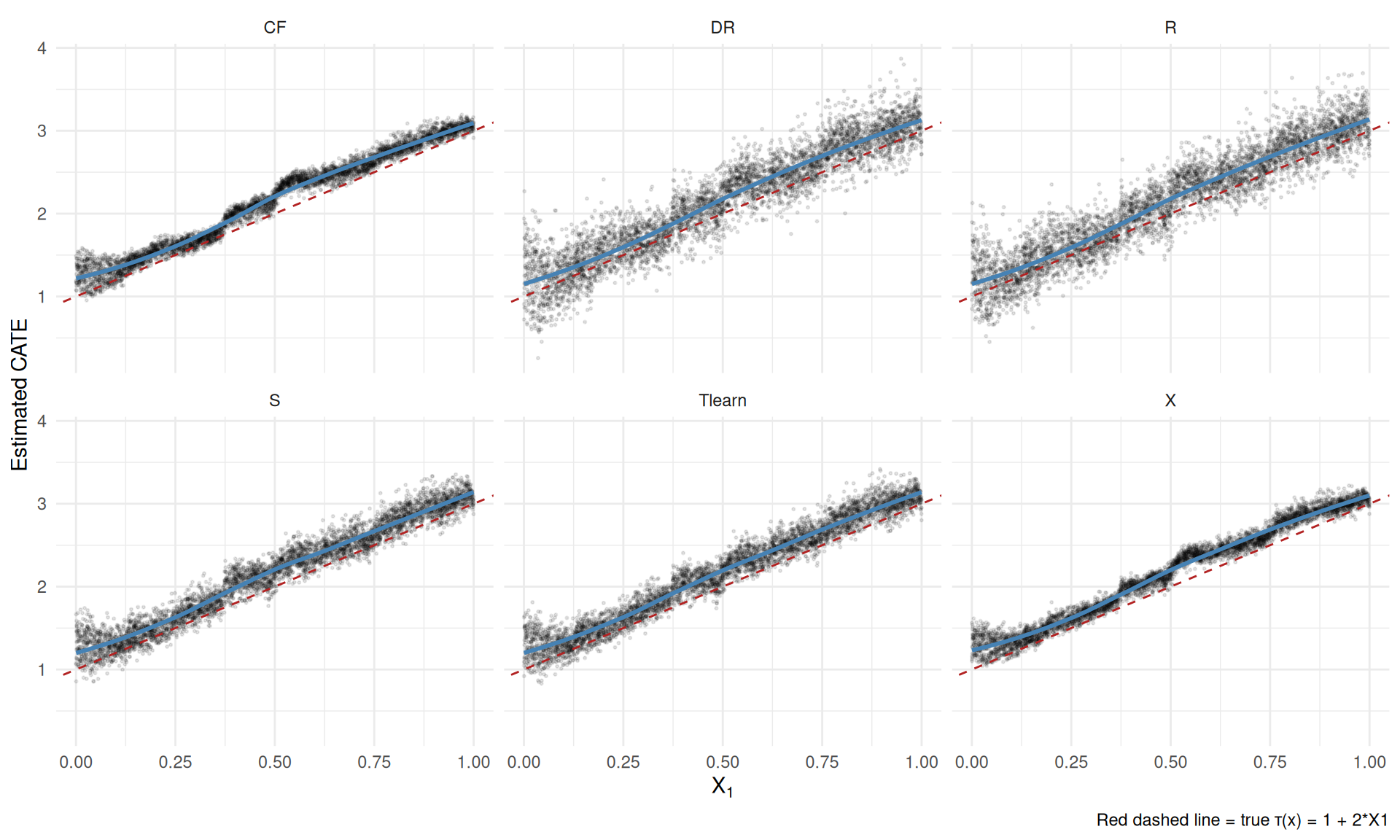

Estimated CATE vs true τ(x) = 1 + 2*X1 for each estimator. Closer to the dashed line = better.

9.4 Best linear projection (BLP)

Even if CATE is nonlinear, we often want a regression-style summary: which covariates are associated with larger effects? The best linear projection of CATE onto \(X\) is

\[ \text{BLP}(X) = \arg\min_{\beta_0, \beta} \mathbb{E}\left[ (\tau(X) - \beta_0 - X'\beta)^2 \right], \]

which grf estimates with valid standard errors:

blp <- best_linear_projection(cf, A = X)
print(blp)

Best linear projection of the conditional average treatment effect.
Confidence intervals are cluster- and heteroskedasticity-robust (HC3):

             Estimate Std. Error t value Pr(>|t|)    
(Intercept)  1.077587   0.119928  8.9853   <2e-16 ***
X1           2.008322   0.104710 19.1798   <2e-16 ***
X2          -0.051931   0.106412 -0.4880   0.6256    
X3          -0.064522   0.102963 -0.6266   0.5309    
X4           0.044172   0.105384  0.4192   0.6751    
X5          -0.115495   0.104588 -1.1043   0.2695    
---
Signif. codes:  0 '***' 0.001 '**' 0.01 '*' 0.05 '.' 0.1 ' ' 1

Here the coefficient on \(X_1\) should be close to 2, and the coefficients on the other variables should be close to 0.

9.5 Variable importance

grf also reports variable importance. It is a rough diagnostic for which variables the forest uses to find heterogeneity.

vi <- variable_importance(cf)
vi_df <- tibble(variable = paste0("X", 1:p), importance = as.numeric(vi)) |>
  arrange(desc(importance))
print(vi_df)

# A tibble: 5 × 2
  variable importance
  <chr>         <dbl>
1 X1           0.725 
2 X4           0.0953
3 X5           0.0703
4 X3           0.0565
5 X2           0.0533

\(X_1\) should be the most important variable in this simulation.

9.6 Policy trees: who should we treat?

A CATE estimate is not yet a policy. If treatment has a cost, the policy question is who should be treated. A policy tree turns estimated treatment effects into a simple treatment rule.

# double_robust_scores() returns an n x 2 matrix of AIPW scores,
# one column per action: Gamma_i(control), Gamma_i(treated)
Gamma <- double_robust_scores(cf)
cost <- 2     # cost of treating one unit, in outcome units

# Net value of each action: control stays as is, treating pays the cost.
# With tau(x) = 1 + 2*x1 in [1, 3], the optimal rule is: treat iff x1 > 0.5.
Gamma[, "treated"] <- Gamma[, "treated"] - cost

# Fit a depth-2 policy tree (shallow for interpretability)
tree <- policy_tree(X, Gamma, depth = 2)
print(tree)

policy_tree object 
Tree depth:  2 
Actions:  1: control 2: treated 
Variable splits: 
(1) split_variable: X1  split_value: 0.626569 
  (2) split_variable: X1  split_value: 0.42175 
    (4) * action: 1 
    (5) * action: 2 
  (3) split_variable: X1  split_value: 0.644418 
    (6) * action: 1 
    (7) * action: 2 

# Recommended action for each unit (1 = control, 2 = treated)
actions <- predict(tree, X)
cat(sprintf("\nTreatment rate under policy tree: %.1f%% (optimal: %.1f%%)\n",
            mean(actions == 2) * 100, mean(X[, 1] > 0.5) * 100))

Treatment rate under policy tree: 56.5% (optimal: 50.5%)

# Value of the learned rule vs treating everyone, both evaluated with
# the same doubly-robust scores
welfare_tree <- mean(ifelse(actions == 2, Gamma[, "treated"], Gamma[, "control"]))
welfare_all  <- mean(Gamma[, "treated"])
cat(sprintf("Estimated welfare: policy tree %.3f vs treat-everyone %.3f (gain %.3f)\n",
            welfare_tree, welfare_all, welfare_tree - welfare_all))

Estimated welfare: policy tree 0.525 vs treat-everyone 0.261 (gain 0.264)

The point of the shallow tree is interpretability. It gives up some flexibility in exchange for a rule that can be inspected. Here the tree splits on \(X_1\) — the true effect modifier — close to the optimal threshold of \(0.5\), and the learned rule beats treat-everyone because units with \(\tau(x) < 2\) are not worth the cost.

For an extended walkthrough of policy trees with IPW and AIPW losses, see the companion blog chapter on policytree. For a comparison of CATE estimators across software ecosystems (including Stata 19’s new cate command), see the Stata CATE blog chapter.

9.7 GATES: sorted group ATEs

GATES (group average treatment effects) is a simple way to report heterogeneity (Chernozhukov et al. 2018). Sort observations by predicted CATE, split them into bins, and estimate the ATE in each bin. If the bin ATEs differ, the heterogeneity is not just a graph. (The same paper’s CLAN — classification analysis — is the natural companion: compare average covariates between the most- and least-affected bins; here that comparison would show high \(X_1\) in the top quintile and low \(X_1\) in the bottom one.)

# Sort by predicted CATE, split into 5 quintiles
nq <- 5
quintile <- cut(tau_cf, breaks = quantile(tau_cf, probs = seq(0, 1, 1/nq)),
                include.lowest = TRUE, labels = FALSE)

# Compute AIPW ATE within each quintile
get_ate <- function(idx) {
  ate <- average_treatment_effect(cf, subset = idx)
  c(est = ate["estimate"], se = ate["std.err"])
}

clan <- t(sapply(1:nq, function(q) get_ate(quintile == q)))
clan_df <- as_tibble(clan) |>
  mutate(quintile = 1:nq,
         lo = est.estimate - 1.96 * se.std.err,
         hi = est.estimate + 1.96 * se.std.err)

knitr::kable(clan_df[, c("quintile", "est.estimate", "se.std.err", "lo", "hi")],
             col.names = c("Quintile", "ATE", "SE", "95% LB", "95% UB"),
             digits = 3,
             caption = "GATES: quintile-specific ATEs sorted by predicted CATE. Heterogeneity is evident if quintile estimates differ.")

GATES: quintile-specific ATEs sorted by predicted CATE. Heterogeneity is evident if quintile estimates differ.

Quintile	ATE	SE	95% LB	95% UB
1	1.263	0.070	1.126	1.400
2	1.517	0.067	1.386	1.649
3	2.106	0.065	1.979	2.234
4	2.274	0.068	2.141	2.408
5	2.810	0.068	2.677	2.943

The bottom and top quintiles should have different estimated ATEs in this simulation. One caveat: the quintiles are formed from the same forest’s (out-of-bag) predictions used to estimate the group ATEs, which mitigates but does not fully remove the bias from grouping and estimating on the same data; for formal inference use a held-out fold or grf::rank_average_treatment_effect().

9.8 Causal forests with panel data

With panel data, unit effects can be correlated with treatment and covariates. A cross-sectional causal forest can then be biased. Two practical fixes are:

1. Demean by fixed effects before running the causal forest.
2. Pass a clusters argument to causal_forest so that observations from the same unit are kept in the same training fold during honest sample-splitting.

set.seed(2024)
n_firms <- 200
n_t     <- 5
n_total <- n_firms * n_t

# Panel data with a unit effect that drives BOTH treatment and the outcome
# (classic fixed-effect confounding; unit_fe is unobserved to the forest)
firm_id  <- rep(1:n_firms, each = n_t)
unit_fe  <- rnorm(n_firms, sd = 1.5)[firm_id]
V1_firm  <- rnorm(n_firms, sd = 1.0)[firm_id]   # firm-level covariate
V1       <- V1_firm + rnorm(n_total, sd = 0.3)  # within-firm variation
W        <- rbinom(n_total, 1, plogis(0.3 * V1_firm + 0.5 * unit_fe))
# True CATE varies linearly with V1
tau_panel <- 0.5 + 1.0 * V1
Y_panel  <- unit_fe + V1 + tau_panel * W + rnorm(n_total)

df_panel <- tibble(firm = firm_id, V1 = V1, W = W, Y = Y_panel)
glimpse(df_panel)

Rows: 1,000
Columns: 4
$ firm <int> 1, 1, 1, 1, 1, 2, 2, 2, 2, 2, 3, 3, 3, 3, 3, 4, 4, 4, 4, 4, 5, 5,…
$ V1   <dbl> 0.60231981, 0.23871074, 0.05916058, -0.24663844, 0.28957601, -0.1…
$ W    <int> 1, 1, 0, 1, 1, 0, 1, 0, 0, 1, 1, 1, 0, 1, 0, 0, 0, 1, 0, 1, 0, 1,…
$ Y    <dbl> 3.99219997, 3.99833174, 1.50594149, 2.51156617, 2.37409880, 0.254…

A naive causal forest ignores the firm effects. Because unit_fe raises both the treatment probability and the outcome, and is not in \(X\), the naive estimate is badly biased upward:

X_panel <- as.matrix(df_panel[, "V1", drop = FALSE])

cf_naive <- causal_forest(X = X_panel, Y = df_panel$Y, W = df_panel$W,
                          num.trees = 1000)
ate_naive <- average_treatment_effect(cf_naive)

cat(sprintf("Naive panel CF ATE: %.3f  (SE = %.3f)\n",
            ate_naive["estimate"], ate_naive["std.err"]))

Naive panel CF ATE: 1.706  (SE = 0.127)

cat(sprintf("True ATE: %.3f\n", mean(tau_panel)))

True ATE: 0.566

Adding clusters = firm keeps a firm’s observations together when grf does the honest sample split. Note what this does and does not do: it makes the honest splitting and the standard errors respect the panel structure, but it does not remove the unobserved-unit-effect confounding — the estimate stays close to the naive one:

cf_clust <- causal_forest(X = X_panel, Y = df_panel$Y, W = df_panel$W,
                          clusters = df_panel$firm,
                          num.trees = 1000)
ate_clust <- average_treatment_effect(cf_clust)

cat(sprintf("Clustered panel CF ATE: %.3f  (SE = %.3f)\n",
            ate_clust["estimate"], ate_clust["std.err"]))

Clustered panel CF ATE: 1.741  (SE = 0.163)

What removes the confounding is the fixed-effect style adjustment: demean \(Y\), \(W\), and \(V_1\) by firm before fitting, which sweeps out unit_fe. A caveat on interpretation: with a demeaned binary treatment \(W_{dm}\), the GRF target is not generally \(\text{mean}(\tau_{panel})\). It is a within-unit, partialled-out contrast whose implicit weighting depends on the distribution of demeaned treatment values. Read the number below as a within-firm residualized treatment effect, not as a drop-in fixed-effect estimate of the same CATE/ATE target as the cross-sectional forest:

df_dm <- df_panel |>
  group_by(firm) |>
  mutate(Y_dm = Y - mean(Y),
         W_dm = W - mean(W),
         V1_dm = V1 - mean(V1)) |>
  ungroup()

cf_fe <- causal_forest(X = as.matrix(df_dm[, "V1_dm"]),
                       Y = df_dm$Y_dm,
                       W = df_dm$W_dm,
                       clusters = df_dm$firm,
                       num.trees = 1000)
ate_fe <- average_treatment_effect(cf_fe)
cat(sprintf("Within-transform CF ATE: %.3f  (SE = %.3f)\n",
            ate_fe["estimate"], ate_fe["std.err"]))

Within-transform CF ATE: 0.577  (SE = 0.103)

The clustered, within-transformed causal forest is a heuristic analogue to a fixed-effect regression with heterogeneous effects, but it does not target the same estimand as a textbook within estimator: properly identified heterogeneous panel effects need stronger assumptions or a dedicated panel/DML construction with an orthogonal score. See the companion blog chapter on causal forests in panel data for an extended simulation study comparing the panel CF to fixed-effect regression and random-effect regression under linear and nonlinear DGPs.

9.9 Summary

• Meta-learners turn outcome-regression tools into CATE estimators.
• Causal forests are the main grf estimator for heterogeneous effects.
• BLP and GATES are useful because they summarize heterogeneity in a way that looks like familiar regression output.
• Policy trees translate CATE estimates into treatment rules.
• In applied work, compare at least two CATE estimators and always report simple heterogeneity summaries, not only a CATE scatterplot.

Chernozhukov, Victor, Mert Demirer, Esther Duflo, and Iván Fernández-Val. 2018. “Generic Machine Learning Inference on Heterogeneous Treatment Effects in Randomized Experiments.” NBER Working Paper 24678.

Kennedy, Edward H. 2020. “Towards Optimal Doubly Robust Estimation of Heterogeneous Causal Effects.” arXiv Preprint arXiv:2004.14497.

Künzel, Sören R., Jasjeet S. Sekhon, Peter J. Bickel, and Bin Yu. 2019. “Metalearners for Estimating Heterogeneous Treatment Effects Using Machine Learning.” Proceedings of the National Academy of Sciences 116 (10): 4156–65.

Nie, Xinkun, and Stefan Wager. 2021. “Quasi-Oracle Estimation of Heterogeneous Treatment Effects.” Biometrika 108 (2): 299–319.