# Causal Discovery: Observed Variables
```{r}
#| include: false
suppressPackageStartupMessages({
library(pcalg)
library(graph)
library(igraph)
library(ggplot2)
library(knitr)
})
# ─── igraph helpers for DAG/CPDAG plotting ───────────────────────────────────
# Convert a graphNEL to a clean igraph.
# For CPDAGs, undirected edges appear as both A→B and B→A in the graphNEL.
# We detect them, deduplicate, and tag them so callers can suppress arrowheads.
graphnel_to_ig <- function(g_nel) {
ig <- igraph::graph_from_graphnel(g_nel)
el <- igraph::as_edgelist(ig)
fwd <- paste(el[,1], el[,2]); rev_ <- paste(el[,2], el[,1])
is_undir <- fwd %in% rev_
# Keep one copy of each undirected pair (smaller-name first)
seen <- character(0); keep <- logical(nrow(el))
for (k in seq_len(nrow(el))) {
if (!is_undir[k]) { keep[k] <- TRUE; next }
key <- paste(sort(c(el[k,1], el[k,2])), collapse="|")
if (key %in% seen) { keep[k] <- FALSE } else { seen <- c(seen, key); keep[k] <- TRUE }
}
ig2 <- igraph::delete_edges(ig, which(!keep))
igraph::E(ig2)$undirected <- is_undir[keep]
igraph::V(ig2)$label.color <- "black"
ig2
}
# Plot a directed/CPDAG igraph with consistent aesthetics.
# layout: precomputed coordinate matrix (reuse across panels for alignment).
plot_ig <- function(g, main = "", layout = NULL, curved = FALSE) {
if (is.null(layout)) layout <- igraph::layout_with_sugiyama(g)$layout
n_e <- igraph::ecount(g)
undir <- if (!is.null(igraph::E(g)$undirected)) igraph::E(g)$undirected else rep(FALSE, n_e)
plot(g,
layout = layout,
main = main,
vertex.size = 26,
vertex.color = "white",
vertex.frame.color = "black",
vertex.label.cex = 0.9,
vertex.label.color = "black",
vertex.label.font = 2,
edge.arrow.size = 0.45,
edge.arrow.mode = ifelse(undir, 0L, 1L),
edge.color = "black",
edge.curved = if (curved) 0.15 else 0)
}
```
Earlier chapters assumed the graph was known, or at least that we could draw
a defensible DAG from subject knowledge. Causal discovery asks what can be
learned about the graph from observational data.
## The Problem
Given $n$ i.i.d. observations of $p$ variables $(X_1, \ldots, X_p)$, we want to recover the directed acyclic graph (DAG) $G$ that generated the data.
There is an important limit: observational data alone cannot distinguish
between DAGs with the same conditional independence structure. The set of
observationally equivalent DAGs is a **Markov equivalence class**. The data
can identify this class, represented by a CPDAG, not necessarily the one true
DAG.
A CPDAG has the same skeleton (undirected edges) as all DAGs in its MEC. Some edges can be oriented (they have the same direction in every member of the MEC); others remain undirected because both directions are consistent with the CI structure.
### Why some edges cannot be oriented
Three DAGs are observationally equivalent — they produce the same set of conditional independences — and therefore indistinguishable from data:
$$X \to Y \to Z \qquad X \leftarrow Y \leftarrow Z \qquad X \leftarrow Y \to Z$$
All three imply $X \perp\!\!\!\perp Z \mid Y$ and no other CI. Their CPDAG shows $X - Y - Z$ with no arrowheads.
The structure $X \to Y \leftarrow Z$ (a **collider** at $Y$) is *not* equivalent: here $X \perp\!\!\!\perp Z$ but $X \not\!\perp\!\!\!\perp Z \mid Y$. Because it has a unique CI signature, the $\to Y \leftarrow$ orientation is identifiable from data. Algorithms orient these colliders; non-collider edges often remain undirected.
### What a CPDAG tells you
A directed edge $X \to Y$ in the CPDAG means: in *every* DAG consistent with the data, $X$ causes $Y$. An undirected edge $X - Y$ means some consistent DAGs have $X \to Y$ and others have $X \leftarrow Y$ — data alone cannot decide.
For causal estimation: once you have a CPDAG, you can use background knowledge (temporal ordering, experimental context) to orient the remaining undirected edges, and then apply identification strategies from earlier chapters.
## Two Discovery Paradigms in R
In R, `pcalg` implements two useful algorithm families:
| Paradigm | Algorithm | Decision rule |
|---|---|---|
| **Constraint-based** | PC (Spirtes & Glymour, 1991) | Remove an edge when a CI test reports independence |
| **Score-based** | GES (Chickering, 2002) | Add/remove/reverse the edge that most improves a model score (BIC) |
Both target the same CPDAG, but they make different mistakes. PC depends on
finite-sample conditional independence tests. GES depends on the score. I
would usually compare both.
## Simulation
We generate a random Gaussian linear DAG using `pcalg::randomDAG` with 8 nodes and edge probability 0.35. Each edge $j \to i$ generates a structural equation
$$X_i = \sum_{j \in \text{pa}(i)} \beta_{ji} X_j + \varepsilon_i, \quad \varepsilon_i \sim N(0,1),$$
with $|\beta_{ji}|$ drawn from $[0.25, 1]$.
```{r}
set.seed(2025)
n_vars <- 8
n_samples <- 2000
edge_prob <- 0.35
labels <- paste0("X", 1:n_vars)
true_dag <- randomDAG(n_vars, prob = edge_prob, lB = 0.25, uB = 1)
graph::nodes(true_dag) <- labels # rename from "1".."8" to "X1".."X8"
data_mat <- rmvDAG(n_samples, true_dag, errDist = "normal")
colnames(data_mat) <- labels
# Adjacency matrix from the true DAG, in the pcalg "ends-at-i" convention:
# entry [i,j] = 1 means an edge ending at i, i.e. j -> i.
adj_true <- t(as(true_dag, "matrix") != 0) * 1
# igraph representation + shared layout for all comparison panels
ig_true <- graphnel_to_ig(true_dag)
dag_layout <- igraph::layout_with_sugiyama(ig_true)$layout
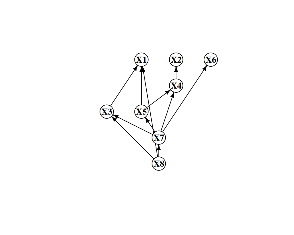
sprintf("Variables: %d Samples: %d True edges: %d",
n_vars, n_samples, sum(adj_true))
```
```{r}
#| label: fig-true-dag
#| fig-cap: "True DAG used for simulation."
#| fig-width: 5
#| fig-height: 4
plot_ig(ig_true, layout = dag_layout)
```
## CI-Test and Score Infrastructure
PC uses a **Fisher-Z conditional independence test** appropriate for Gaussian data. Given the partial correlation $\hat\rho_{XY \mid Z}$, the test statistic is
$$T = \sqrt{n - |Z| - 3} \cdot \operatorname{atanh}(\hat\rho_{XY \mid Z}) \;\sim\; N(0,1) \quad \text{under } H_0: X \perp\!\!\!\perp Y \mid Z.$$
**Choosing the significance level** $\alpha$ involves a bias–variance tradeoff on the skeleton:
An edge is *removed* whenever a CI test fails to reject independence
($p \ge \alpha$), so $\alpha$ controls how easily edges are deleted:
- **Low $\alpha$ (e.g., 0.001)**: independence is rarely rejected, so more
tests "find" independence and more edges are removed. Sparser skeleton;
risks discarding real but weak edges.
- **High $\alpha$ (e.g., 0.05)**: independence is rejected more often, so
fewer edges are removed. Denser skeleton; risks retaining spurious edges.
With $n = 2000$ and $p = 8$ we use $\alpha = 0.01$, a common default.
GES does not use a significance level. It selects the graph that *minimizes*
the **Gaussian BIC**
$$\text{BIC}(G) = -2 \,\ell(\hat\theta; G) + |G| \log n$$
(equivalently, maximizes the penalized log-likelihood
$\ell - \tfrac{|G|}{2}\log n$), which penalizes graph complexity directly.
Implemented in `pcalg` as `GaussL0penObsScore`.
We wrap `gaussCItest` in a counter to track exactly how many CI tests PC calls:
```{r}
make_counted_ci <- function(suff_stat) {
  count <- 0L
  ci <- function(x, y, S, suffStat) {
    count <<- count + 1L
    gaussCItest(x, y, S, suffStat)
  }
  list(ci = ci, count = function() count)
}

suff_stat <- list(C = cor(data_mat), n = n_samples)
```
## PC Algorithm
The **PC algorithm** (Spirtes & Glymour, 1991) starts from a complete undirected graph and removes edges whenever a conditional independence is found. It searches for separating sets $Z$ of increasing size, conditioning on subsets of the current neighbors. After skeleton discovery, Meek's rules orient as many edges as possible.
**How it works, step by step:**
1. Start with a complete undirected graph (every pair connected).
2. For each pair $(X, Y)$, test $X \perp\!\!\!\perp Y \mid Z$ for all $Z \subseteq \text{neighbors}(X) \setminus \{Y\}$, starting with $|Z| = 0$. Remove the edge if any such test passes.
3. Repeat with conditioning sets of increasing size until no new edges are removed.
4. Identify colliders: if $X - Z - Y$ and $X, Y$ non-adjacent, orient as $X \to Z \leftarrow Y$ only if $Z$ was not in the separating set of $X$ and $Y$.
5. Apply Meek's orientation rules to propagate orientations without creating new colliders or cycles.
```{r}
sig_level <- 0.01

ci_pc  <- make_counted_ci(suff_stat)
pc_fit <- pc(suffStat = suff_stat,
             indepTest = ci_pc$ci,
             labels = labels,
             alpha = sig_level,
             verbose = FALSE)

cpdag_pc <- pc_fit@graph
ci_tests_pc <- ci_pc$count()
```
::: {.callout-note}
**Reading the output: F1 scores**
The **F1 score** is the harmonic mean of precision and recall, ranging from 0 (worst) to 1 (perfect).
- **Skeleton F1** measures whether the algorithm found the right edges regardless of direction. An edge is a true positive if it exists in both the estimated skeleton and the true one.
- **CPDAG F1** is stricter: a directed edge $X \to Y$ is only a true positive if the true DAG also has $X \to Y$; an undirected edge $X - Y$ counts as correct if the true DAG has *either* direction.
A high skeleton F1 with lower CPDAG F1 means the algorithm found the right adjacencies but oriented some of them incorrectly. **Caveat:** this is an *orientation-error-only* score -- leaving a truly directed edge undirected is never penalized, only actively wrong directions are. It is therefore not a standard CPDAG accuracy metric (which would also penalize unresolved/uncompelled orientations), and it can flatter an algorithm that simply declines to orient edges. Read it as "of the orientations made, how many are right," not "how much of the true CPDAG was recovered."
:::
```{r}
# Helper: extract directed adjacency matrix from a graphNEL CPDAG.
# pcalg convention: amat[i,j] = 1 means an edge that ENDS at i,
# i.e. a directed edge j -> i (or one endpoint of an undirected edge).
amat_from_graph <- function(g) {
  # as(g, "matrix")[i,j] = 1 means i -> j (from->to). Transpose so that
  # [i,j] = 1 means an edge ending at i (j -> i), matching adj_true's
  # convention; otherwise CPDAG-F1 compares opposite orientations.
  m <- t(as(g, "matrix") != 0)
  storage.mode(m) <- "integer"
  m
}

# Skeleton: symmetrize (edge exists either way).
amat_to_skel <- function(amat) (amat | t(amat)) * 1L

# F1 scores: skeleton F1 (ignore direction) and CPDAG F1
# (directed edge in estimate must match a directed edge in the truth;
#  undirected in estimate matches either direction in truth).
# CAUTION if reusing this function elsewhere: the CPDAG-F1 component is
# orientation-error-only -- it never penalizes leaving a truly directed edge
# undirected, only actively wrong orientations. It is not a standard CPDAG
# accuracy metric and can flatter an algorithm that declines to orient
# edges. See the discussion above this function for what it does and does
# not measure.
f1_scores <- function(amat_true, amat_est) {
  skel_t <- amat_to_skel(amat_true)
  skel_e <- amat_to_skel(amat_est)
  diag(skel_t) <- diag(skel_e) <- 0
  tp <- sum(skel_t & skel_e) / 2
  fp <- sum(!skel_t & skel_e) / 2
  fn <- sum(skel_t & !skel_e) / 2
  f1_skel <- if (tp == 0) 0 else 2 * tp / (2 * tp + fp + fn)

  # CPDAG F1: walk ordered pairs (i,j) with i < j
  tp <- fp <- fn <- 0
  p <- nrow(amat_true)
  for (i in seq_len(p - 1)) for (j in seq.int(i + 1, p)) {
    t_ij <- amat_true[j, i] == 1   # truth has i -> j?
    t_ji <- amat_true[i, j] == 1   # truth has j -> i?
    e_ij <- amat_est[j, i] == 1
    e_ji <- amat_est[i, j] == 1
    if (!t_ij && !t_ji && !e_ij && !e_ji) next
    truth_undirected <- t_ij && t_ji
    est_undirected   <- e_ij && e_ji
    has_t <- t_ij || t_ji
    has_e <- e_ij || e_ji
    if (has_t && has_e) {
      if (est_undirected || truth_undirected ||
          (t_ij == e_ij && t_ji == e_ji)) {
        tp <- tp + 1
      } else {
        fp <- fp + 1; fn <- fn + 1
      }
    } else if (has_e) {
      fp <- fp + 1
    } else {
      fn <- fn + 1
    }
  }
  f1_cpdag <- if (tp == 0) 0 else 2 * tp / (2 * tp + fp + fn)

  c(skeleton = f1_skel, cpdag = f1_cpdag)
}

amat_pc  <- amat_from_graph(cpdag_pc)
f1_pc    <- f1_scores(adj_true, amat_pc)
ig_cpdag_pc <- graphnel_to_ig(cpdag_pc)

sprintf("PC:    skeleton F1 = %.3f   CPDAG F1 = %.3f   CI tests = %d",
        f1_pc["skeleton"], f1_pc["cpdag"], ci_tests_pc)
```
**Computational complexity:** In the worst case PC tests all subsets of neighbors, giving exponential growth with the maximum degree. In sparse graphs this is manageable; in dense graphs it becomes prohibitive.
## GES Algorithm
**GES** (Greedy Equivalence Search; Chickering, 2002) uses a different strategy. Instead of testing independences and removing edges, it searches the space of CPDAGs by adding and then removing edges that improve a model score. Under faithfulness and a consistent score such as BIC, GES recovers the true CPDAG as $n \to \infty$.
**How it works, step by step:**
1. **Forward phase.** Start from the empty graph. At each step, add the single edge whose addition most increases the BIC score, restricted to additions that stay within a CPDAG. Stop when no addition improves the score.
2. **Backward phase.** From the forward-phase output, remove the single edge whose removal most increases the score. Stop when no removal improves the score.
The whole search operates on CPDAGs (equivalence classes), not individual DAGs, so it explores a much smaller space than naïve DAG search.
```{r}
score_ges <- new("GaussL0penObsScore", data_mat)
ges_fit   <- ges(score_ges, verbose = FALSE)
cpdag_ges <- as(ges_fit$essgraph, "graphNEL")

amat_ges  <- amat_from_graph(cpdag_ges)
f1_ges    <- f1_scores(adj_true, amat_ges)
ig_cpdag_ges <- graphnel_to_ig(cpdag_ges)

sprintf("GES:   skeleton F1 = %.3f   CPDAG F1 = %.3f   (score-based, no CI tests)",
        f1_ges["skeleton"], f1_ges["cpdag"])
```
PC and GES fail differently. In PC, one wrong CI decision can affect later
orientation decisions. In GES, a wrong score move is usually more local.
## Comparison
::: {.callout-note}
**Reading the CPDAG figure**
In the side-by-side graph display:
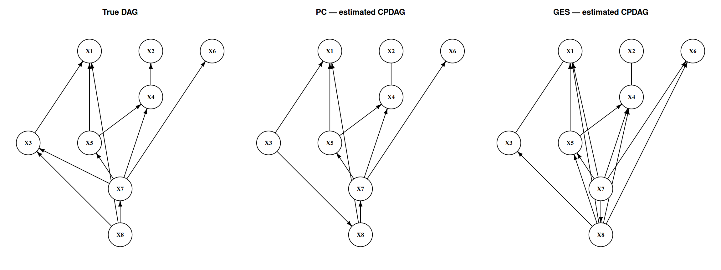
- A **directed edge** $X_i \to X_j$ means this orientation is invariant across all equivalent DAGs.
- An **undirected edge** $X_i - X_j$ in the CPDAG display represents an *unoriented* edge: both $X_i \to X_j$ and $X_i \leftarrow X_j$ are statistically equivalent. This is **not** a hidden common cause — it means the data cannot determine direction.
- A **missing edge** means the algorithm found a conditional independence separating those two variables.
Compare the estimated CPDAGs to the true DAG: extra edges are false positives; missing edges are false negatives.
:::
```{r}
#| label: tbl-comparison
#| tbl-cap: "Algorithm comparison on the simulated 8-node DAG (n = 2000, alpha = 0.01)"
kable(data.frame(
  Algorithm   = c("PC", "GES"),
  Paradigm    = c("Constraint-based", "Score-based"),
  Skeleton_F1 = round(c(f1_pc["skeleton"], f1_ges["skeleton"]), 3),
  CPDAG_F1    = round(c(f1_pc["cpdag"],    f1_ges["cpdag"]),    3),
  CI_Tests    = c(ci_tests_pc, NA)
), row.names = FALSE)
```
```{r}
#| label: fig-cpdags
#| fig-cap: "True DAG vs. estimated CPDAGs. Arrows denote oriented edges; lines without arrowheads are unoriented (both directions are CI-equivalent)."
#| fig-width: 12
#| fig-height: 4.5
op <- par(mfrow = c(1, 3), mar = c(1, 1, 3, 1))
plot_ig(ig_true,     layout = dag_layout, main = "True DAG")
plot_ig(ig_cpdag_pc, layout = dag_layout, main = "PC — estimated CPDAG")
plot_ig(ig_cpdag_ges,layout = dag_layout, main = "GES — estimated CPDAG")
par(op)
```
::: {.callout-note}
**Interpreting the comparison table**
- **Skeleton F1** is the primary metric for comparing algorithms: it measures edge recovery independent of orientation, since orientation accuracy is bounded by the MEC.
- **CPDAG F1** additionally rewards correctly oriented edges and penalizes wrongly oriented ones (leaving an edge undirected is not penalized under our scoring).
- **CI tests** is reported only for PC — GES is score-based and does not perform CI tests.
On this dataset PC comes out ahead on both metrics: GES's backward phase prunes or merges a few true adjacencies, which costs it skeleton F1 and, through the lost edges, CPDAG F1 as well. There is no general ranking — both algorithms target the *same* CPDAG, and the BIC score carries no orientation information beyond the conditional-independence structure (all DAGs in one Markov equivalence class receive the same score). Which one gets closer in finite samples depends on the DGP, the sample size, and the tuning ($\alpha$ vs. the BIC penalty).
:::
## Monte Carlo Evaluation
A single dataset can be lucky. We average over 100 replications to get stable estimates.
**What to look for in the MC results:**
- The **mean skeleton F1** is the headline: how often does each algorithm recover the true adjacencies?
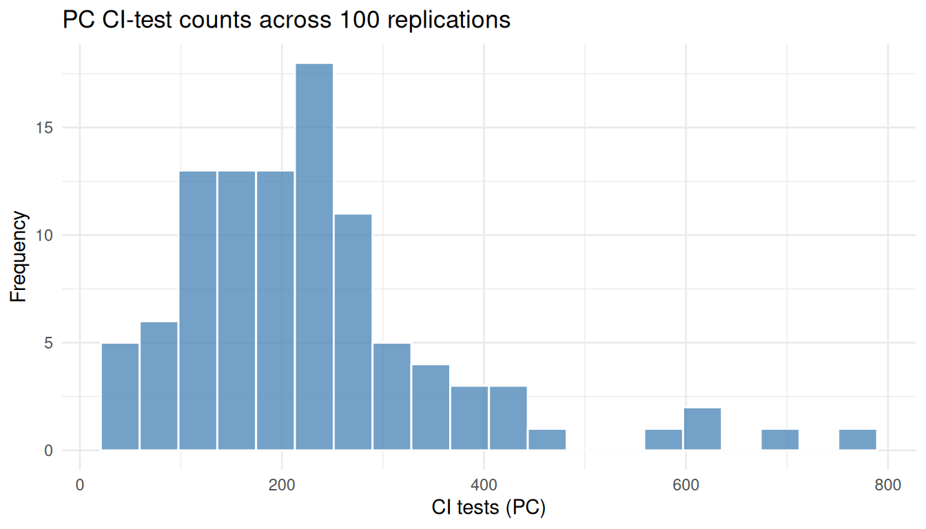
- The distribution of **CI test counts** (shown in @fig-mc-ci) tracks PC's computational variability; GES has no analogous quantity, so we plot PC alone.
- High variance in F1 across replications suggests the algorithms are sensitive to the particular random graph.
```{r}
#| cache: true
evaluate_once <- function(seed, n_vars = 8, n_samples = 2000,
                          edge_prob = 0.35, sig = 0.01) {
  set.seed(seed)
  dag      <- randomDAG(n_vars, prob = edge_prob, lB = 0.25, uB = 1)
  labs     <- paste0("X", 1:n_vars)
  graph::nodes(dag) <- labs
  d        <- rmvDAG(n_samples, dag, errDist = "normal")
  colnames(d) <- labs
  adj      <- t(as(dag, "matrix") != 0) * 1L
  ss       <- list(C = cor(d), n = n_samples)

  ci       <- make_counted_ci(ss)
  pc_f     <- pc(ss, ci$ci, labels = labs, alpha = sig, verbose = FALSE)
  amat_p   <- amat_from_graph(pc_f@graph)

  ges_f    <- ges(new("GaussL0penObsScore", d), verbose = FALSE)
  amat_g   <- amat_from_graph(as(ges_f$essgraph, "graphNEL"))

  f_p <- f1_scores(adj, amat_p); f_g <- f1_scores(adj, amat_g)
  c(f1_skel_pc  = f_p["skeleton"], f1_skel_ges = f_g["skeleton"],
    f1_cpdag_pc = f_p["cpdag"],    f1_cpdag_ges = f_g["cpdag"],
    ci_pc       = ci$count())
}

mc <- as.data.frame(t(sapply(1:100, evaluate_once)))
names(mc) <- c("f1_skel_pc","f1_skel_ges","f1_cpdag_pc","f1_cpdag_ges","ci_pc")

mc_summary <- data.frame(
  Method      = c("PC", "GES"),
  Skeleton_F1 = round(c(mean(mc$f1_skel_pc),  mean(mc$f1_skel_ges)),  3),
  CPDAG_F1    = round(c(mean(mc$f1_cpdag_pc), mean(mc$f1_cpdag_ges)), 3),
  CI_Tests    = c(round(mean(mc$ci_pc), 1), NA)
)
kable(mc_summary,
      caption = "Monte Carlo averages (100 replications, n = 2000, p = 8)",
      row.names = FALSE)
```
```{r}
#| label: fig-mc-ci
#| fig-cap: "Distribution of PC's CI-test counts across 100 replications. The spread reflects how PC's cost depends on the realized graph density and the order of CI decisions."
#| fig-width: 7
#| fig-height: 4
ggplot(mc, aes(x = ci_pc)) +
  geom_histogram(bins = 20, fill = "steelblue", alpha = 0.75, color = "white") +
  labs(x = "CI tests (PC)", y = "Frequency",
       title = "PC CI-test counts across 100 replications") +
  theme_minimal()
```
## Real Data: Student Performance in PISA
The simulation had a luxury real research never does: a known true DAG, so we
could score recovery with F1. On real data there is **no ground truth**, so the
questions change. Instead of "how close is the estimate to the truth?" we ask:
do PC and GES *agree*; what can *background knowledge* orient; and is the
structure *stable* under resampling?
We illustrate on the OECD's **PISA 2022** assessment, restricted to **United
States** students and six variables with a clear substantive ordering.
| Node | Meaning | Role |
|---|---|---|
| `HISEI` | Highest parental occupational status (ISEI) | Family background |
| `HOMEPOS` | Home possessions index | Family background |
| `IMMIG` | Immigration status (1 native … 3 first-gen) | Demographic |
| `GRADE` | Grade relative to modal grade for age | Schooling |
| `GENDER` | 1 = female, 0 = male | Demographic |
| `MATH` | Mean of the 10 mathematics plausible values | Outcome |
```{r}
pisa <- read.csv("data/pisa_usa2022.csv")
Xp   <- as.matrix(pisa[, c("HISEI","HOMEPOS","IMMIG","GRADE","GENDER","MATH")])
wp   <- pisa$W
plabs <- colnames(Xp)
sprintf("Students (complete cases): %d", nrow(Xp))
```
::: {.callout-note}
**Three honesty caveats**, kept explicit:
- **Plausible values.** Each student's ability is reported as 10 plausible
values (posterior draws), not one score. We use their mean, understating the
measurement variance; a full treatment runs discovery on each PV and pools.
- **Categorical-as-Gaussian.** `IMMIG`, `GRADE`, `GENDER` are discrete; Fisher-Z
assumes joint Gaussianity — a standard but imperfect approximation.
- **One country, one wave.** Pooling would inject country/time structure that
appears as spurious edges unless modelled as extra nodes.
:::
### Respecting the survey design
PISA is not a simple random sample — students carry final weights `W_FSTUWT`.
The CI tests and the score are functions of the **covariance matrix** and a
**sample size**, so we supply design-consistent inputs: a **weighted
covariance/correlation** matrix, and **Kish's effective sample size**
$n_{\text{eff}} = (\sum_i w_i)^2 / \sum_i w_i^2$.
```{r}
cwp   <- cov.wt(Xp, wt = wp, cor = TRUE)   # design-weighted moments
Cwp   <- cwp$cor
Sigp  <- cwp$cov
neff  <- sum(wp)^2 / sum(wp^2)
sprintf("Raw n = %d   Kish effective n = %.0f", nrow(Xp), neff)
```
```{r}
#| label: tbl-pisa-cor
#| tbl-cap: "Design-weighted correlation matrix (PISA 2022, USA)."
kable(round(Cwp, 2))
```
### Two algorithms on the weighted data
PC consumes the weighted correlation and effective $n$ directly. GES is
score-based and needs a data matrix, so we build a synthetic sample of
$n_{\text{eff}}$ rows whose empirical covariance equals the design-weighted
$\Sigma_w$ exactly (a Cholesky recolour) — a device to feed the *same* second
moments into a score that expects raw data, adding no information beyond
$\Sigma_w$.
This is a **moment-based approximation to the PISA design, not
design-exact causal discovery.** The weighted covariance plus Kish's
$n_{\text{eff}}$ captures the final weights but not the full
stratification and clustering of the design, and it ignores
plausible-value (imputation) uncertainty in the achievement scores.
Treat the recovered graph as a weighted-moment exploration, and do not
read the effective-$n$ CI tests as exact design-based inference.
```{r}
# Synthetic matrix with covariance == Sigp exactly, neff rows
m_eff <- round(neff)
set.seed(1)
Zp <- scale(matrix(rnorm(m_eff * ncol(Xp)), m_eff), center = TRUE, scale = FALSE)
Zp <- Zp %*% solve(chol(cov(Zp)))     # whiten
Xw <- Zp %*% chol(Sigp)               # recolour to weighted covariance
Xw <- sweep(Xw, 2, cwp$center, "+")
colnames(Xw) <- plabs

pc_pisa   <- pc(list(C = Cwp, n = neff), indepTest = gaussCItest,
                labels = plabs, alpha = 0.01)
amat_pcp  <- amat_from_graph(pc_pisa@graph)

ges_pisa  <- ges(new("GaussL0penObsScore", Xw))
cpdag_gesp<- as(ges_pisa$essgraph, "graphNEL")
amat_gesp <- amat_from_graph(cpdag_gesp)

skp <- amat_to_skel(amat_pcp); skg <- amat_to_skel(amat_gesp)
diag(skp) <- diag(skg) <- 0
sprintf("Skeleton edges — PC: %d   GES: %d   in both: %d",
        sum(skp)/2, sum(skg)/2, sum(skp & skg)/2)
```
```{r}
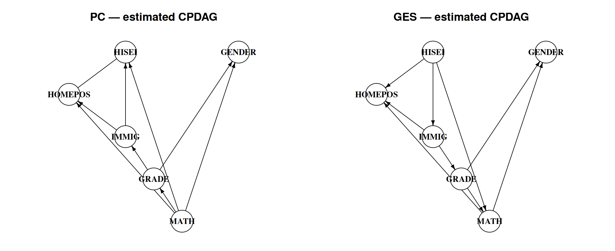
#| label: fig-pisa-cpdags
#| fig-cap: "Estimated CPDAGs from PC and GES on PISA 2022 (USA). Arrows are oriented edges; plain lines are unoriented. There is no true-DAG panel — on real data we have no ground truth."
#| fig-width: 11
#| fig-height: 4.5
ig_pcp  <- graphnel_to_ig(pc_pisa@graph)
ig_gesp <- graphnel_to_ig(cpdag_gesp)
lay_p   <- igraph::layout_with_sugiyama(ig_pcp)$layout
op <- par(mfrow = c(1, 2), mar = c(1, 1, 3, 1))
plot_ig(ig_pcp,  layout = lay_p, main = "PC — estimated CPDAG")
plot_ig(ig_gesp, layout = lay_p, main = "GES — estimated CPDAG")
par(op)
```
::: {.callout-important}
**Read the disagreement, not just the agreement.** A purely data-driven score
may orient an edge as `MATH → HISEI` — a child's test score causing their
parent's occupational status (GES does exactly this in the right panel). That
is causally backwards, and the data cannot protect us: which direction this
edge takes is not identifiable from observational data alone, so the
orientation the algorithm prints reflects its (possibly mistaken) v-structure
and score decisions under misspecification, not evidence about the true
direction. This is exactly why background knowledge is not optional.
:::
### Orienting with background knowledge
Sex and immigration background are fixed at birth; family socioeconomic status
is established long before the test; grade precedes the assessment; the score is
the outcome. That gives a **tier ordering**
$$
\{\text{GENDER}, \text{IMMIG}\} \prec \{\text{HISEI}, \text{HOMEPOS}\}
\prec \text{GRADE} \prec \text{MATH}.
$$
A cross-tier edge must point earlier→later; a within-tier edge the ordering
cannot decide. We impose this on the discovered **skeleton**, because the
ordering is knowledge we hold independently of how the data oriented things.
```{r}
tier_p <- c(HISEI = 1, HOMEPOS = 1, IMMIG = 0, GRADE = 2, GENDER = 0, MATH = 3)[plabs]
skel_p <- amat_to_skel(amat_pcp)

edges_df <- data.frame(); undir_flag <- logical(0)
pp <- length(plabs)
for (i in seq_len(pp-1)) for (j in seq.int(i+1, pp)) {
  if (skel_p[i, j] == 0) next
  a <- plabs[i]; b <- plabs[j]
  if (tier_p[a] == tier_p[b]) {
    edges_df <- rbind(edges_df, data.frame(from = a, to = b)); undir_flag <- c(undir_flag, TRUE)
  } else {
    lo <- if (tier_p[a] < tier_p[b]) a else b
    hi <- if (tier_p[a] < tier_p[b]) b else a
    edges_df <- rbind(edges_df, data.frame(from = lo, to = hi)); undir_flag <- c(undir_flag, FALSE)
  }
}
ig_orient <- igraph::graph_from_data_frame(edges_df, vertices = plabs)
igraph::E(ig_orient)$undirected <- undir_flag
```
::: {.callout-warning}
**Where data-driven orientation disagreed with us.** Left to itself, PC
oriented `HISEI → IMMIG` and `HOMEPOS → IMMIG` — parental status and home
possessions causing immigration background, which our tier ordering puts the
other way round. GES did something worse with a different edge: it oriented
`GRADE → IMMIG`, schooling causing immigration status (PC got that one
right). These mistakes come from v-structure and score decisions made under
misspecification; the data is not informative about these directions.
Imposing the tier order overrides them. The lesson: **never ship a
discovered orientation you have prior reason to disbelieve**.
:::
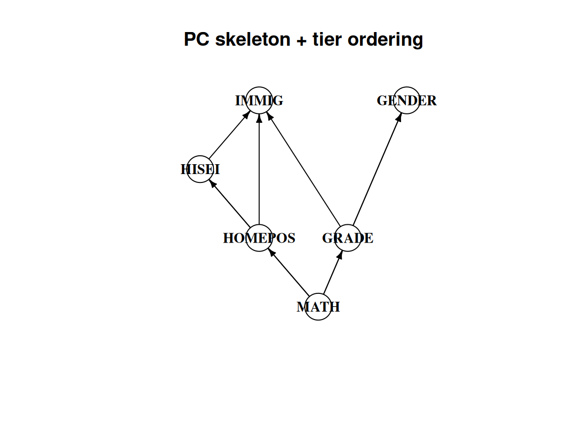
```{r}
#| label: fig-pisa-oriented
#| fig-cap: "PC skeleton oriented by the temporal/logical tiers. Cross-tier edges point earlier-to-later; HISEI–HOMEPOS stays undirected (same tier)."
#| fig-width: 6
#| fig-height: 4.5
lay_or <- igraph::layout_with_sugiyama(ig_orient)$layout
plot_ig(ig_orient, layout = lay_or, main = "PC skeleton + tier ordering")
```
Every edge into `MATH` is now a candidate causal parent of achievement — the
bridge from discovery to estimation (back-door adjustment, e.g. on the parents
of the chosen treatment variable). The only edge the ordering leaves
undirected, `HISEI – HOMEPOS`, is
two same-tier measures of family background that temporal logic cannot separate.
### Stability: does the skeleton survive resampling?
A single fit can be lucky. We resample students with replacement, re-estimate
the **weighted** PC skeleton, and record how often each edge appears.
```{r}
#| cache: true
B_pisa <- 200
boot_once <- function(b) {
  set.seed(1000 + b)
  idx <- sample.int(nrow(Xp), replace = TRUE)
  Xb  <- Xp[idx, ]; wb <- wp[idx]
  cwb <- cov.wt(Xb, wt = wb, cor = TRUE)
  neff_b <- sum(wb)^2 / sum(wb^2)
  fit <- tryCatch(pc(list(C = cwb$cor, n = neff_b), indepTest = gaussCItest,
                     labels = plabs, alpha = 0.01), error = function(e) NULL)
  if (is.null(fit)) return(NULL)
  amat_to_skel(amat_from_graph(fit@graph))
}
ncores <- max(1, parallel::detectCores() - 1)
skels  <- parallel::mclapply(seq_len(B_pisa), boot_once, mc.cores = ncores)
skels  <- skels[!vapply(skels, is.null, logical(1))]
edge_freq <- Reduce(`+`, skels) / length(skels)
```
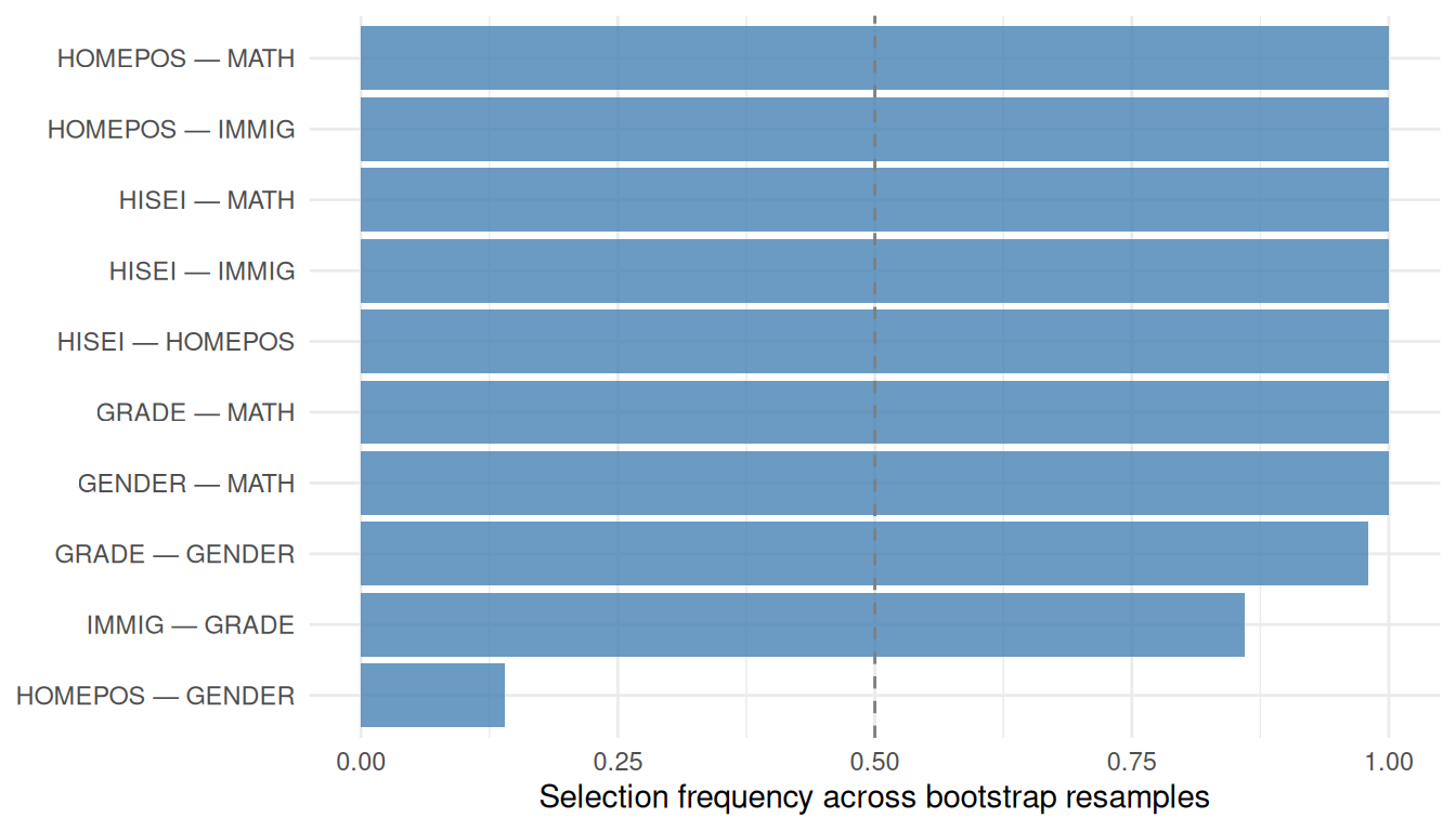
```{r}
#| label: fig-pisa-stability
#| fig-cap: "Bootstrap edge-selection frequency (weighted PC, 200 resamples). Edges near 1.0 are robust; near 0.5 are sample-dependent."
#| fig-width: 7
#| fig-height: 4
pairs_df <- do.call(rbind, lapply(seq_len(pp-1), function(i)
  do.call(rbind, lapply(seq.int(i+1, pp), function(j)
    data.frame(Edge = paste(plabs[i], "—", plabs[j]),
               Frequency = round(edge_freq[i, j], 2))))))
pairs_df <- pairs_df[pairs_df$Frequency > 0, ]
ggplot(pairs_df, aes(x = reorder(Edge, Frequency), y = Frequency)) +
  geom_col(fill = "steelblue", alpha = 0.8) +
  geom_hline(yintercept = 0.5, linetype = "dashed", colour = "grey50") +
  coord_flip() + ylim(0, 1) +
  labs(x = NULL, y = "Selection frequency across bootstrap resamples") +
  theme_minimal()
```
The family-background→math edges (`HISEI`, `HOMEPOS`) are the most stable
features: the SES gradient in achievement is not an artefact. On real data,
causal discovery is best read as **hypothesis generation** — it proposes a
skeleton and the orientations the data support, which you then reconcile with
subject-matter knowledge before estimating effects.
## Summary
PC and GES target the same Markov equivalence class. PC uses conditional
independence tests; GES uses model fit. If they agree on the skeleton, that
is reassuring. If they disagree, check sample size, model assumptions, and
possible faithfulness problems.
**From CPDAG to causal estimation:** Once a CPDAG is in hand, the workflow continues as follows:
1. **Use background knowledge to orient undirected edges.** Temporal ordering is the most common source: if $X$ is measured before $Y$, the edge must be $X \to Y$. Domain expertise, experimental context, or exclusion restrictions can orient others.
2. **Check identifiability.** With a fully oriented DAG, apply the backdoor, front-door, or ID algorithm to determine whether the effect of interest is identifiable.
3. **Estimate.** Use the identified functional with the estimators from earlier chapters (RA, IPW, AIPW, TMLE).
If some edges remain undirected after exhausting background knowledge, you can either report the CPDAG and bound the estimand over the equivalence class, or collect additional interventional data to break the remaining equivalences.
::: {.callout-note}
**What cannot be recovered from observational data alone**
Both algorithms identify the CPDAG, not necessarily the true DAG. Some edge
directions require extra assumptions, temporal ordering, or interventional
data.
The next chapter addresses a harder problem: recovering the causal skeleton when some variables are *unobserved*.
:::