3  DAGs, ADMGs, Identification, and Estimation

The potential-outcomes chapter asked when an observed data set can tell us about \(E[Y(1)-Y(0)]\). Graphs give one way to state the assumptions behind the answer. A graph records which variables are allowed to cause other variables, and whether some observed variables may share unobserved common causes. Once the graph is stated, identification is a graph problem. Estimation comes after that: estimate the functional that the graph identified.

I use dagitty for graphs and backdoor adjustment, causaleffect for the general Pearl-Shpitser ID algorithm, and small direct estimators for the examples. The goal is to keep the order clear: graph first, identified functional second, estimator third.

3.1 DAGs and ADMGs

The graphical machinery in this chapter is Pearl’s (2009). A directed acyclic graph, or DAG, has directed arrows such as X -> A. In causal work, an arrow means a direct causal relation is allowed by the model. Absence of an arrow is also a substantive assumption.

An acyclic directed mixed graph, or ADMG, adds bidirected arrows such as A <-> Y. ADMGs are the graphs the general identification theory of Shpitser and Pearl (2006) operates on, and causaleffect (Tikka, Hyttinen, and Karvanen 2019) implements that theory. A bidirected edge represents an unobserved common cause. This is useful because many econometric applications have variables we cannot measure: ability, preferences, latent health, firm quality, and so on.

The graph is not an estimator. It is a compact statement of assumptions. The workflow is:

1. write down a DAG or ADMG;
2. ask whether the target effect is identified;
3. estimate the identified functional from data.

3.2 A DAG: Backdoor Adjustment

The criterion is Pearl’s (1995), and the adjustment sets below are found with dagitty (Textor et al. 2016). Start with a simple observational study. A is treatment, Y is the outcome, and X is an observed confounder:

g_dag <- dagitty("dag {
  X -> A
  X -> Y
  A -> Y
}")
coordinates(g_dag) <- list(
  x = c(X = 1, A = 0, Y = 2),
  y = c(X = 1, A = 0, Y = 0)
)

ggdag(g_dag) + theme_dag_blank()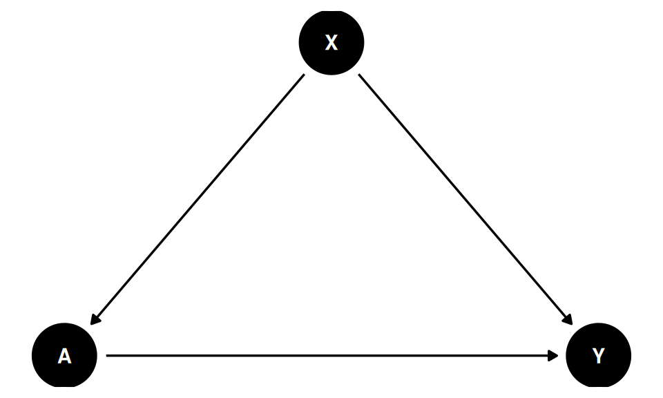

Figure 3.1: Backdoor DAG: X is an observed confounder of A → Y.

The graph says X affects both treatment and outcome. It also says there is no unobserved common cause between A and Y after we condition on X. In this case the treatment effect is identifiable by backdoor adjustment.

adj_sets <- adjustmentSets(g_dag, exposure = "A", outcome = "Y")
adj_sets

{ X }

The adjustment set is \(\{X\}\). Under this graph,

\[ E[Y(a)] = E_X\{E(Y \mid A=a, X)\}. \tag{3.1}\]

So the graph has translated a causal query into an observed-data functional.

3.3 Estimating the DAG Effect with AIPW

The augmented inverse-probability-weighted estimator comes from Robins, Rotnitzky and Zhao (1994); Bang and Robins (2005) give the form used here. We simulate data that match this graph, so we can check whether an estimator built from the identified functional recovers an effect we already know.

We draw \(n = 400\) observations. The confounder is \(X \sim N(0,1)\). Treatment is \(A \sim \text{Bernoulli}(\Lambda(-0.2 + 0.8X))\), with \(\Lambda\) the logistic function, so a higher \(X\) makes treatment more likely. The outcome is \(Y = 1 + 1.5A + 0.7X + 0.3\varepsilon\) with \(\varepsilon \sim N(0,1)\). The effect is constant across units, so the ATE is 1.5.

set.seed(2026)

logistic <- function(x) 1 / (1 + exp(-x))

n  <- 400
X  <- rnorm(n)
pA <- logistic(-0.2 + 0.8 * X)
A  <- as.numeric(runif(n) < pA)
Y  <- 1 + 1.5 * A + 0.7 * X + 0.3 * rnorm(n)

df_dag <- data.frame(X = X, A = A, Y = Y)
head(df_dag)

            X A          Y
1  0.52058907 0  1.6530538
2 -1.07969076 0  0.1907760
3  0.13923812 0  1.0984536
4 -0.08474878 0  1.0941604
5 -0.66663962 1  1.8965341
6 -2.51608903 0 -0.8245336

The analyst sees only \(X\), \(A\) and \(Y\). Because \(X\) raises both the chance of treatment and the outcome, a raw contrast of \(Y\) by \(A\) overstates the effect.

Because the graph is backdoor-identified, use AIPW with the adjustment set the graph chose. The function below implements the AIPW point estimate and an EIF-based standard error.

aipw_backdoor <- function(data, treatment, outcome, adjust) {
  fmla_y <- as.formula(paste0(outcome, " ~ ", treatment, " * (",
                              paste(adjust, collapse = " + "), ")"))
  fmla_a <- as.formula(paste0(treatment, " ~ ",
                              paste(adjust, collapse = " + ")))

  mu_fit <- lm(fmla_y, data = data)
  pi_fit <- glm(fmla_a, data = data, family = binomial())

  d1 <- data; d1[[treatment]] <- 1
  d0 <- data; d0[[treatment]] <- 0
  mu1 <- predict(mu_fit, newdata = d1)
  mu0 <- predict(mu_fit, newdata = d0)
  pi1 <- predict(pi_fit, newdata = data, type = "response")

  w  <- data[[treatment]]; y <- data[[outcome]]
  if1 <- w     * (y - mu1) / pi1       + mu1
  if0 <- (1-w) * (y - mu0) / (1 - pi1) + mu0
  psi  <- if1 - if0

  est  <- mean(psi)
  se   <- sd(psi) / sqrt(length(psi))
  ci   <- est + c(-1, 1) * qnorm(0.975) * se
  data.frame(estimand = "Backdoor ACE",
             estimate = round(est, 4),
             lower_95 = round(ci[1], 4),
             upper_95 = round(ci[2], 4),
             se       = round(se, 4))
}

aipw_backdoor(df_dag, "A", "Y", adjust = "X") |> kable()

estimand	estimate	lower_95	upper_95	se
Backdoor ACE	1.4886	1.427	1.5502	0.0314

AIPW returns 1.4886 with an influence-function standard error of 0.0314, and the 95% interval \([1.427, 1.550]\) covers the true ACE of 1.5. The graph chose the adjustment set and the estimator used that set.

The standard error here, sd(psi) / sqrt(n), is the influence-function standard error of the AIPW estimator. It is asymptotically valid when the nuisance functions (\(\mu\) and \(\pi\)) are regular parametric fits, as they are here. With flexible machine-learning nuisances it is not valid as written: you then need cross-fitting (sample splitting) so the nuisance estimates are independent of the fold being evaluated, and the variance should still be computed from the efficient influence function (or by bootstrap). Treating a full-sample ML AIPW estimate with this plug-in SE will generally understate uncertainty.

3.4 An ADMG: Front-Door Identification

The front-door criterion is also due to Pearl (1995). Now suppose treatment and outcome share an unobserved common cause. A simple adjustment argument no longer works. The front-door ADMG has a mediator M that transmits the effect of A to Y, while A and Y are hidden-confounded:

g_fd <- dagitty("dag {
  A -> M
  M -> Y
  A <-> Y
}")
coordinates(g_fd) <- list(
  x = c(A = 0, M = 1, Y = 2),
  y = c(A = 0, M = 0, Y = 0)
)

ggdag(g_fd) + theme_dag_blank()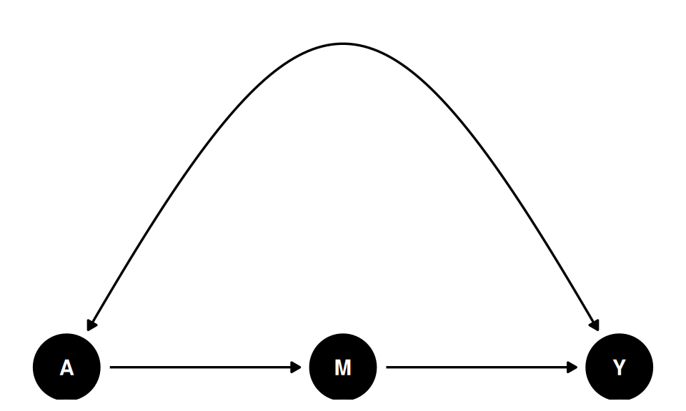

Figure 3.2: Front-door ADMG: A and Y share an unobserved common cause (curved bidirected edge), but the effect propagates through the mediator M.

The bidirected edge A <-> Y means that ordinary backdoor adjustment is not available. Indeed dagitty reports no adjustment set:

sets_fd <- adjustmentSets(g_fd, exposure = "A", outcome = "Y")
# An empty dagitty adjustment-set list prints nothing at all, which is easy to
# mistake for a chunk that failed to run. Report the count explicitly.
cat("Valid backdoor adjustment sets:", length(sets_fd), "\n")

Valid backdoor adjustment sets: 0 

There are none. No set of observed variables blocks the confounding, because the confounder is not observed.

But the effect is still identified by the front-door criterion (Pearl, 1995). I call the Pearl-Shpitser ID algorithm in causaleffect to obtain the symbolic expression. The function wants the graph as an igraph object with bidirected edges encoded as two directed edges marked description = "U". It returns the expression as a LaTeX string, so the printed line below is LaTeX source, not a typeset formula:

g_fd_ig <- graph_from_literal(A -+ M, M -+ Y, A -+ Y, Y -+ A)
# Mark the A<->Y bidirected edge (encoded as the two directed edges A->Y and
# Y->A) by endpoint name rather than by hardcoded edge index -- igraph's
# internal edge ordering after graph_from_literal() is not part of its
# documented contract, so indices like c(2, 4) can silently point at the
# wrong edges if igraph's internals, the vertex/edge creation order, or the
# package version ever changes.
edge_ends <- ends(g_fd_ig, E(g_fd_ig))
confounded <- (edge_ends[, 1] == "A" & edge_ends[, 2] == "Y") |
              (edge_ends[, 1] == "Y" & edge_ends[, 2] == "A")
E(g_fd_ig)$description[confounded] <- "U"
expr_fd <- causal.effect(y = "Y", x = "A", G = g_fd_ig, simp = TRUE)
cat(expr_fd, "\n")

\sum_{M}P(M|A)\left(\sum_{A}P(Y|A,M)P(A)\right) 

The expression \(\sum_M P(M\mid A)\sum_{A'} P(Y\mid A', M) P(A')\) is precisely the front-door formula.

3.5 Estimating the ADMG Effect with the Front-Door Formula

We simulate a front-door setting so we can compare the front-door estimate against a truth we derive below.

We draw \(n = 400\) observations. The latent confounder is \(U \sim N(0,1)\). Treatment is \(A \sim \text{Bernoulli}(\Lambda(-0.1 + 0.8U))\), the mediator is \(M \sim \text{Bernoulli}(\Lambda(-0.4 + 1.2A))\), and the outcome is \(Y \sim \text{Bernoulli}(\Lambda(-1.0 + 0.9M + 0.7U))\). All three observed variables are binary. \(U\) is not in the observed data; it is what the bidirected edge A <-> Y stands for. Two features make the front-door criterion apply: \(U\) enters \(A\) and \(Y\) but not \(M\), and \(A\) reaches \(Y\) only through \(M\).

set.seed(2027)

n     <- 400
U     <- rnorm(n)
A_fd  <- as.numeric(runif(n) < logistic(-0.1 + 0.8 * U))
M     <- as.numeric(runif(n) < logistic(-0.4 + 1.2 * A_fd))
Y_fd  <- as.numeric(runif(n) < logistic(-1.0 + 0.9 * M + 0.7 * U))

df_fd <- data.frame(A = A_fd, M = M, Y = Y_fd)
head(df_fd)

  A M Y
1 0 0 0
2 0 1 1
3 1 1 1
4 1 1 1
5 0 1 1
6 1 0 0

The front-door point estimator is a direct evaluation of the identification expression:

\[ E[Y(a)] = \sum_m P(M=m\mid A=a)\sum_{a'} P(Y=1\mid A=a', M=m) P(A=a'). \tag{3.2}\]

The DGP has a known truth. Under \(do(A=a)\) the mediator is \(M \sim \text{Bern}(\Lambda(-0.4 + 1.2a))\) while \(U\) keeps its marginal \(N(0,1)\) distribution, so

\[ \tau = \big[\Lambda(0.8) - \Lambda(-0.4)\big]\; \big[g(-0.1) - g(-1.0)\big], \qquad g(c) = E_U\big[\Lambda(c + 0.7U)\big], \tag{3.3}\]

which evaluates to \(0.2887 \times 0.1894 = 0.0547\). The naive contrast \(E[Y\mid A=1]-E[Y\mid A=0]\) equals \(0.158\) in the population this DGP defines — almost three times the causal effect, because \(U\) raises both the chance of treatment and the outcome. That gap is what the front-door step removes. The table below reports the sample version of the naive contrast alongside the front-door estimate.

For binary \(A\), \(M\), \(Y\) we plug sample proportions into that formula, and take the standard error from 500 bootstrap resamples:

front_door_ace <- function(data) {
  pA <- mean(data$A)
  p_marginal_A <- c("0" = 1 - pA, "1" = pA)

  # P(M | A): rows indexed by A, columns by M
  pM_given_A <- prop.table(table(data$A, data$M), margin = 1)
  # P(Y=1 | A, M)
  pY_given_AM <- with(data, tapply(Y, list(A, M), mean))

  # E[Y(a)] for a in {0, 1}
  ey_do <- function(a) {
    m_levels <- as.numeric(colnames(pM_given_A))
    sum(sapply(m_levels, function(m) {
      mar <- pM_given_A[as.character(a), as.character(m)]
      inner <- sum(sapply(c(0, 1), function(ap)
        pY_given_AM[as.character(ap), as.character(m)] *
          p_marginal_A[as.character(ap)]))
      mar * inner
    }))
  }
  ey_do(1) - ey_do(0)
}

# Bootstrap for SE
set.seed(99)
B   <- 500
boot_ace <- replicate(B, {
  idx <- sample.int(nrow(df_fd), replace = TRUE)
  front_door_ace(df_fd[idx, ])
})

est_fd <- front_door_ace(df_fd)
se_fd  <- sd(boot_ace)
ci_fd  <- est_fd + c(-1, 1) * qnorm(0.975) * se_fd

naive_fd <- mean(df_fd$Y[df_fd$A == 1]) - mean(df_fd$Y[df_fd$A == 0])

data.frame(estimand = c("Naive E[Y|A=1] - E[Y|A=0]", "Front-door ACE", "Truth"),
           estimate = round(c(naive_fd, est_fd, 0.0547), 4),
           lower_95 = c(NA, round(ci_fd[1], 4), NA),
           upper_95 = c(NA, round(ci_fd[2], 4), NA),
           se       = c(NA, round(se_fd, 4), NA)) |> kable()

estimand	estimate	lower_95	upper_95	se
Naive E[Y|A=1] - E[Y|A=0]	0.1395	NA	NA	NA
Front-door ACE	0.0775	0.0403	0.1146	0.0189
Truth	0.0547	NA	NA	NA

The naive contrast is 0.1395, more than twice the true 0.0547. The front-door estimate is 0.0775 with a bootstrap standard error of 0.0189, and its 95% interval \([0.040, 0.115]\) covers the truth. The confounding bias is removed; what is left is sampling noise, and the interval is wide relative to an effect of 0.05 because the formula estimates seven proportions from 400 binary observations: \(P(A=1)\), the two mediator probabilities \(P(M=1 \mid A=a)\), and the four outcome probabilities \(P(Y=1 \mid A=a, M=m)\).

3.6 General ID Algorithm

Backdoor adjustment and the front-door formula are useful because they are easy to estimate. ADMGs can be more general. The Pearl-Shpitser ID algorithm asks the broader question:

Can P(Y | do(A)) be written using only the observed joint law P(V)?

The algorithm works recursively:

1. remove variables that are not ancestors of the outcome;
2. add interventions that are irrelevant after graph surgery;
3. split the remaining graph into bidirected districts;
4. identify each district as a factor of the observed law, if possible;
5. return a hedge witness when no such reduction is possible.

For the front-door graph, the general ID algorithm succeeds and returns the same front-door formula we obtained above. For more complex ADMGs it may yield novel functionals that no named estimator covers — this is where the plug-in approach is essential.

3.7 When the Graph Says No

The bow graph has both a direct causal edge and unobserved confounding between the same two variables:

g_bow <- dagitty("dag {
  A -> Y
  A <-> Y
}")
coordinates(g_bow) <- list(
  x = c(A = 0, Y = 1),
  y = c(A = 0, Y = 0)
)

ggdag(g_bow) + theme_dag_blank()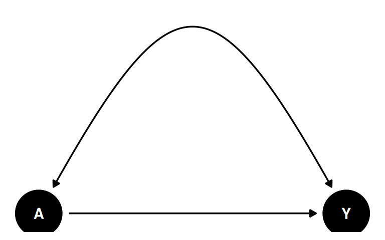

Figure 3.3: Bow ADMG: a direct edge A → Y plus a bidirected A ↔︎ Y. The effect is not identified.

The effect of A on Y is not identified in this ADMG. The observed association mixes the direct causal effect with the latent common cause.

g_bow_ig <- graph_from_literal(A -+ Y, Y -+ A)
g_bow_ig <- set_edge_attr(g_bow_ig, "description",
                          index = c(1, 2), value = "U")
g_bow_ig <- add_edges(g_bow_ig, c("A", "Y"))   # add the direct A -> Y

result <- tryCatch(
  causal.effect(y = "Y", x = "A", G = g_bow_ig, simp = TRUE),
  error = function(e) paste("Not identifiable:", conditionMessage(e))
)
result

[1] "Not identifiable: Not identifiable."

causaleffect raises an error message indicating the effect is not identifiable.

3.8 Practical Workflow

For applied work, a useful workflow is:

1. write the graph before looking at estimates;
2. use bidirected edges for latent common causes;
3. ask dagitty::adjustmentSets(graph, exposure, outcome) — if non-empty, you have a backdoor route;
4. if no adjustment set exists, call causaleffect::causal.effect(y, x, G) — if it returns an expression, the effect is identified by a more general route; if it errors, the effect is not identified in this ADMG;
5. estimate using AIPW for backdoor effects, the front-door formula when the algorithm returns that pattern, or a plug-in evaluation of the symbolic expression for general ID functionals;
6. report the graph and the identification route along with the estimate.

Bang, Heejung, and James M. Robins. 2005. “Doubly Robust Estimation in Missing Data and Causal Inference Models.” Biometrics 61 (4): 962–73.

Pearl, Judea. 1995. “Causal Diagrams for Empirical Research.” Biometrika 82 (4): 669–88.

———. 2009. Causality: Models, Reasoning, and Inference. 2nd ed. Cambridge University Press.

Robins, James M., Andrea Rotnitzky, and Lue Ping Zhao. 1994. “Estimation of Regression Coefficients When Some Regressors Are Not Always Observed.” Journal of the American Statistical Association 89 (427): 846–66.

Shpitser, Ilya, and Judea Pearl. 2006. “Identification of Joint Interventional Distributions in Recursive Semi-Markovian Causal Models.” In Proceedings of the 21st National Conference on Artificial Intelligence (AAAI), 1219–26.

Textor, Johannes, Benito van der Zander, Mark S. Gilthorpe, Maciej Liśkiewicz, and George T. H. Ellison. 2016. “Robust Causal Inference Using Directed Acyclic Graphs: The R Package dagitty.” International Journal of Epidemiology 45 (6): 1887–94.

Tikka, Santtu, Antti Hyttinen, and Juha Karvanen. 2019. “Causal Effect Identification from Multiple Incomplete Data Sources: A General Search-Based Approach.” Journal of Statistical Software 99 (5).