---
title: "Modeling variation, not just the mean, in Likert-scale data"
date: "2026-07-16"
---
```{r}
#| label: setup
#| include: false
# Loaded here (uncached) rather than inside a cache: true chunk below, so
# these packages are attached to the search path even when downstream
# chunks are skipped and lazy-loaded from a valid cache.
library(ggplot2)
library(dplyr)
library(brms)
```
## Modeling the spread, not the mean
Usually we regress a Likert item on covariates and model only its mean. A 1--7
satisfaction item, a 1--5 agreement item, a peer rating --- we ask what moves
the average.
But many questions are about the spread. Do evaluators agree more about some
employees than others? Does one group of raters disagree more than another?
Does a training program tighten the distribution of responses, or only shift
its center?
The natural move is to compute a spread for each unit --- each subject's
ratings across raters, each respondent's answers across items --- and regress
*that* on covariates, the way we regress a mean. On a bounded scale, that move
breaks. This chapter is about why it breaks, and what to do instead.
## The ceiling is exact, not empirical
On a scale with a hard floor and ceiling, the largest variance a set of
responses can have depends on where their mean sits. This is not a tendency in
typical data. It is a mathematical fact, true for any distribution on a
bounded interval.
Take any $X$ confined to $[a,b]$. Both $(X-a)$ and $(b-X)$ are non-negative for
every draw, so their product is too:
$$(X-a)(b-X) \geq 0 \quad \text{for every } X \in [a,b].$$
Take expectations, expand, and substitute into
$\text{Var}(X) = E[X^2] - \mu^2$ (with $\mu = E[X]$):
$$\text{Var}(X) \leq (a+b)\mu - ab - \mu^2 = (\mu - a)(b - \mu).$$
This is the **Bhatia--Davis inequality** (Bhatia and Davis 2000). In words: fix
the mean, and the variance cannot exceed a value set entirely by that mean and
the scale's endpoints. Equality is reached, not just approached --- put all the
mass at the two endpoints, $P(X=a) = (b-\mu)/(b-a)$ and $P(X=b) =
(\mu-a)/(b-a)$, and the variance hits $(\mu-a)(b-\mu)$ exactly. That is the most
polarized a set of responses can be, given the mean.
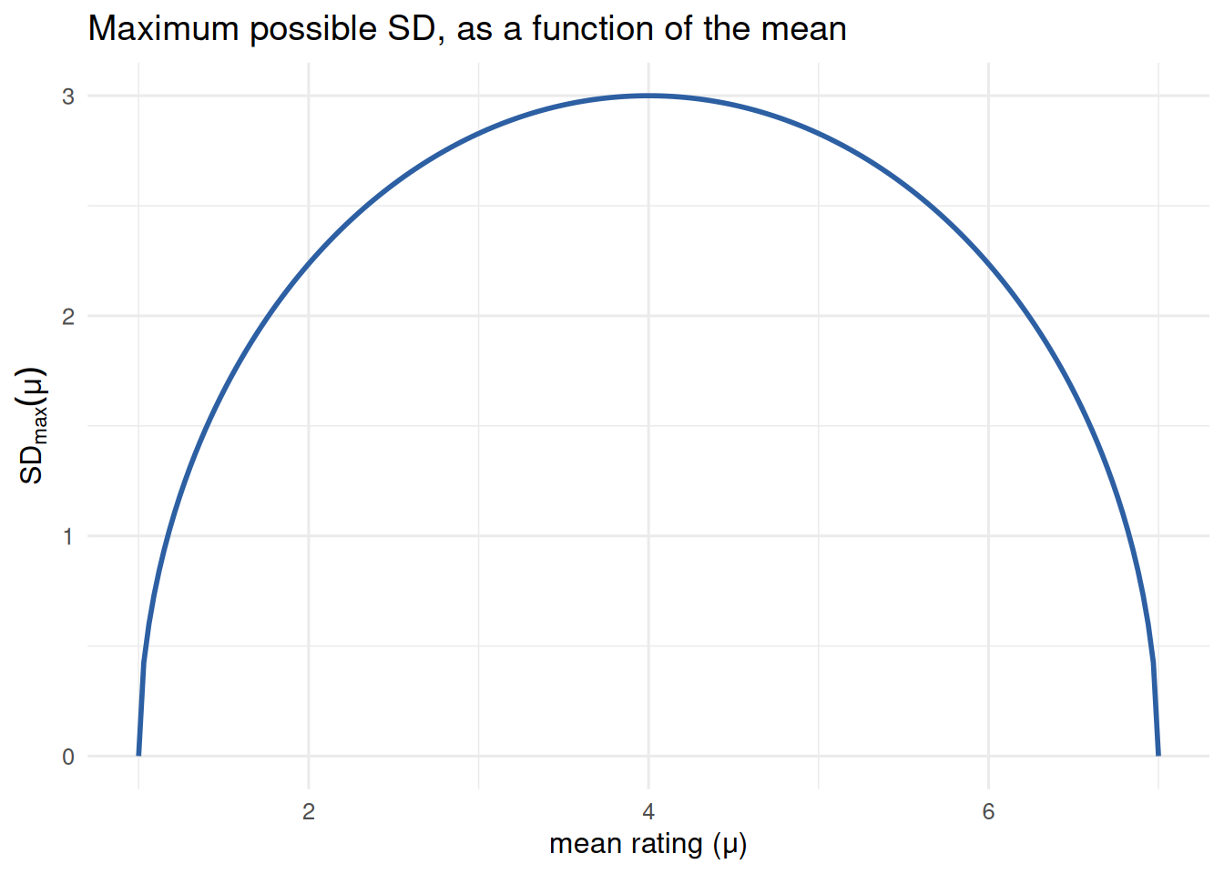
On a 1--7 item that is
$$\text{SD}_{\max}(\mu) = \sqrt{(\mu-1)(7-\mu)},$$
a downward parabola. It is widest at the midpoint ($\mu=4$, where
$\text{SD}_{\max}=3$) and pinched to exactly zero at both ends. A respondent
whose raters all pick 7 has zero disagreement, by definition. There is nowhere
else for a rating to go.
```{r}
#| label: bound-curve
#| echo: true
#| message: false
#| warning: false
#| fig-cap: "The mechanical ceiling on SD, given the mean, for a 1--7 scale."
mu_grid <- seq(1, 7, length.out = 200)
sd_max <- sqrt(pmax((mu_grid - 1) * (7 - mu_grid), 0))
ggplot(data.frame(mu = mu_grid, sd_max = sd_max), aes(mu, sd_max)) +
geom_line(linewidth = 1, color = "#2d5fa3") +
labs(x = "mean rating (μ)", y = expression(SD[max](mu)),
title = "Maximum possible SD, as a function of the mean") +
theme_minimal(base_size = 12)
```
The consequence is direct. Two groups whose *means* differ have different
*ceilings* on their SD, whether or not their true dispersion differs at all.
And skew makes this the common case, not a corner case. Satisfaction items,
performance ratings, and health scales usually sit near one end of the scale
--- exactly where the curve is steepest, and where raw SD comparisons mislead
most.
::: {.callout-note}
## A finite-sample refinement
The curve is the *population* bound. For a finite sample of $n$ real numbers
with mean $\mu$, the true maximum is tighter still. Ellis (2025) gives it
exactly as $\text{Var}_{\max}(n,\mu) = (\mu-1)(7-\mu) - \tfrac{36}{n}a(1-a)$,
where $a$ is the fractional part of $n(\mu-1)/6$; this sits between
$(\mu-1)(7-\mu) - 9/n$ and $(\mu-1)(7-\mu)$. At $n=5$ raters that is up to 1.8
points$^2$ of extra slack --- worth knowing when only a handful of people rate
each unit, since the population curve then understates how tight the real
ceiling is.
:::
## Dividing by the mean does not fix it
The first instinct is to divide the SD by the mean, the way you would for a
coefficient of variation. It does not work here. That correction is built for a
*different* mechanism --- variance scaling proportionally with the mean, as in
count data --- not a ceiling that pinches to zero at *both* ends.
$\text{SD}_{\max}(\mu)/\mu$ is still a curve: zero at $\mu=1$, a peak of $0.75$
at $\mu=4$, back to zero at $\mu=7$. Dividing by the mean does not remove the
mean-dependence. It relabels it.
## The right idea: spread after removing the ceiling effect
Every fix worth having does the same thing --- measure dispersion *after*
dividing out the ceiling. Beta regression names this directly. Rescale the
outcome to $(0,1)$ (e.g. $(y-1)/6$ for a 1--7 item) and parameterize by a mean
$\mu$ and a precision $\varphi$ (Ferrari and Cribari-Neto 2004; `betareg` in
Cribari-Neto and Zeileis 2010). On the 1--7 scale,
$$\text{Var}(Y) = \frac{(\mu-1)(7-\mu)}{1+\varphi}
\qquad \Longrightarrow \qquad
\varphi = \frac{(\mu-1)(7-\mu)}{\text{Var}(Y)} - 1.$$
Set $\varphi = 0$ and this *is* the Bhatia--Davis bound. In words: $\varphi$ is
dispersion measured after the boundary is divided out, so $\varphi \sim
\text{group}$ compares spread without inheriting the ceiling the way raw SD
does.
$\varphi$ itself is awkward to report --- it lives on $(0,\infty)$ with no
natural reference point. Its bounded twin is easier:
$$R := \frac{\text{Var}(Y)}{\text{Var}_{\max}(\mu)} = \frac{1}{1+\varphi}.$$
By Bhatia--Davis, $\text{Var}(Y) \leq \text{Var}_{\max}(\mu)$ for *any*
distribution on $[1,7]$, not just Beta ones, so $R \in [0,1]$ always, with no
distributional assumption. $R=1$ means a subject's raters are as polarized as
the ceiling allows, given their mean; $R=0$ means perfect consensus. It reads
like a percentage because it is one.
Two costs come with it. First, it is a continuous model grafted onto discrete,
ordinal data --- a 1--7 response is not a continuous proportion. Second, both
forms put a rater-estimated variance in a denominator, and that variance comes
from only a handful of raters. For $\varphi$ the denominator is
$\text{Var}(Y)$: when a few raters agree by chance --- more likely near the
ceiling, where most of the sample lives --- $\text{Var}(Y) \to 0$ and $\varphi
\to \infty$. For $R$ the denominator is $\text{Var}_{\max}(\mu)$, which is zero
whenever the mean sits at a scale endpoint; if all raters pick 7, then
$\text{Var}(Y)$ and $\text{Var}_{\max}$ vanish together and $R = 0/0$ is
undefined outright. We return to this in the worked example, because it bites
hard.
## Two models: one with the boundary, one without
### Gaussian location-scale model (MELSM)
The location-scale model is the fix people reach for first. Model the mean as
usual, and *also* model the residual SD as a function of covariates.
```r
library(brms)
fit_gaussian <- brm(
bf(rating ~ group + (1 | subject),
sigma ~ group), # model the SD, not just the mean
data = df, family = gaussian()
)
```
`brms` puts a log link on `sigma`, so the `group` coefficient on the `sigma`
part is a difference in *log*-SD. Exponentiate it for an SD ratio between
groups.
The catch is fatal for our question. A Gaussian model has no boundary in it. It
does not know the scale stops at 1 and 7. So it cannot tell "this group's raters
genuinely agree more" from "this group's mean sits closer to the ceiling." Both
produce the identical signature in the fitted `sigma`.
### Ordinal cumulative-probit MELSM: put the boundary inside the model
The clean fix treats the 1--7 response as what it is: a discretized slice of a
latent continuous trait, cut by six ordered thresholds.
Posit an unobserved continuous $Y_i^*$ behind each rating,
$$Y_i^* = \eta_i + \sigma_i \epsilon_i, \qquad \epsilon_i \sim N(0,1),$$
where $\eta_i$ is the linear predictor for *location* (`group` plus a subject
random intercept, say) and $\sigma_i$ is the latent residual SD, which we also
let depend on covariates. The observed rating is $Y_i^*$ coarsened at six fixed
thresholds $\theta_1 < \cdots < \theta_6$ (with $\theta_0=-\infty$,
$\theta_7=\infty$):
$$Y_i = k \iff \theta_{k-1} < Y_i^* \leq \theta_k.$$
So the cumulative probability is
$$P(Y_i \leq k) = P\!\left(\epsilon_i \leq \frac{\theta_k - \eta_i}{\sigma_i}\right)
= \Phi\!\left(\frac{\theta_k - \eta_i}{\sigma_i}\right),$$
with $\Phi$ the standard normal CDF, for the probit link. Write $\text{disc}_i
:= 1/\sigma_i$ and this is `brms`'s parameterization exactly:
$$P(Y_i \leq k) = \Phi\bigl(\text{disc}_i\,(\theta_k - \eta_i)\bigr).$$
In words: discrimination is the reciprocal of the latent residual SD. Not an
analogy --- an algebraic identity, reached by rescaling the argument of $\Phi$
rather than dividing by $\sigma_i$ directly. Letting `disc` depend on covariates
is the ordinal analogue of `sigma ~ group`, written in reciprocal form: a
positivity-friendly way to let dispersion vary ($\text{disc} > 0$ everywhere,
with no constraint on $\sigma_i$ itself). `brms` puts a log link on `disc`, so
`disc ~ 0 + group` means $\log(\text{disc}_i) = \gamma_{\text{group}[i]}$ --- a
group difference in *log*-discrimination, parallel to the Gaussian log-SD
coefficient (Bürkner and Vuorre 2019).
```r
fit_ordinal <- brm(
bf(rating ~ group + (1 | subject),
disc ~ 0 + group), # log(disc) = 0 + group; disc = 1 / latent SD
data = df, family = cumulative("probit"), init = 0,
prior = c(
prior(constant(0), class = "b", coef = "groupA", dpar = "disc"),
prior(normal(0, 1), class = "b", coef = "groupB", dpar = "disc")
)
)
```
The `constant(0)` prior pins the reference group's *log*-discrimination
--- the linear predictor $\gamma_A$, not $\text{disc}$ itself --- at zero, so
$\text{disc}_A = \exp(0) = 1$ and its latent SD is $1/\text{disc}_A = 1$.
(Fixing $\gamma_A=0$ is what makes `disc = 1` and `SD = 1` coincide for the
reference group; it is not a claim that discrimination is zero, which would
mean an infinite latent SD.) Only $\gamma_B$ is estimated: $\text{disc}_B =
\exp(\gamma_B)$, so $\gamma_B=0$ means identical dispersion, $\gamma_B>0$ means
Group B is *more* discriminating (a *smaller* latent SD), and $\gamma_B<0$ the
reverse. The boundary is now explicit --- six estimated cutpoints on an
*unbounded* latent scale --- so a group whose mean sits near 7 no longer shows
a tighter latent SD by mechanics alone.
### What belongs in the dispersion submodel?
A fair question: why does the dispersion side carry only `group`, when the mean
model might carry more? Should the two not mirror each other? Not by default.
They answer different questions. The mean model asks what predicts the average
rating. The dispersion model asks what predicts the spread. A covariate earns
its place on each side on its own merits.
In this chapter's simulation `group` is the only variable in the
data-generating process, so there is nothing else *to* include, on either side.
In real data the choice is substantive, and getting it wrong has a familiar
cost. Suppose some covariate $Z$ (rater experience, item wording, a
subject-level trait) genuinely shifts dispersion and is correlated with `group`,
but is left out of the dispersion submodel. Its effect is absorbed into the
`group` coefficient on `sigma` (or `disc`, or $\varphi$) --- omitted-variable
bias for the *variance*, exactly analogous to the ordinary one for the mean. The
remedy is the same one you already use on the mean side: include the covariates
you have a substantive reason to think shift dispersion, and give that choice
the same scrutiny --- neither copying the mean formula reflexively nor stripping
the dispersion submodel to the one comparison you happen to care about.
### Four candidates, side by side
Two questions separate the approaches: does it remove the mechanical ceiling,
and does it stay stable when only a handful of raters rate each unit? Only one
passes both.
| Approach | Removes the mechanical ceiling? | Stable at $n\approx5$ raters? |
|---|---|---|
| SD $/$ mean | No --- still a curve in $\mu$, just a different one | No --- inherits raw SD's sampling noise |
| Hand-built $R = \text{Var}/\text{Var}_{\max}$ | Yes, by construction | No --- the denominator collapses near the ceiling, and $R$ is undefined at a scale endpoint |
| Gaussian MELSM's `sigma` | No --- no boundary in the model, so it inherits the confound | Yes --- the joint likelihood pools across units |
| Ordinal MELSM's `disc` | Yes --- the boundary lives in six estimated thresholds | Yes --- the joint likelihood pools across units |
The useful way to remember it: $R$ is the right idea computed the wrong way,
and the Gaussian MELSM is the wrong idea computed the right way --- stable and
precise, but blind to the boundary, so it reports the ceiling artifact as a
confident finding. `disc` is the same idea as $R$ --- spread with the ceiling
effect removed --- estimated coherently inside one model. The worked example
shows all of this.
## Worked example: same dispersion, different means
Simulate two groups of 100 subjects each, 6 raters per subject. Both groups'
raters draw from a **latent** continuous opinion with the *same* true SD
($\sigma = 1$) --- there is no real disagreement difference to find. Group A's
latent mean sits high (near the ceiling once discretized); Group B's sits in
the middle of the range.
```{r}
#| label: simulate
#| echo: true
#| message: false
#| warning: false
#| cache: true
set.seed(42)
n_per_group <- 100
n_raters <- 6
sigma_true <- 1.0 # SAME latent SD in both groups -- no real difference
mu_A <- 2.4 # group A's latent mean sits near the ceiling
mu_B <- 0.6 # group B's sits mid-range
subjects <- data.frame(
subject = 1:(2 * n_per_group),
group = rep(c("A", "B"), each = n_per_group),
mu = rep(c(mu_A, mu_B), each = n_per_group)
)
df <- subjects[rep(seq_len(nrow(subjects)), each = n_raters), ]
df$latent <- rnorm(nrow(df), mean = df$mu, sd = sigma_true)
# six fixed cutpoints -> seven observed categories, 1 through 7
cuts <- c(-2, -1.2, -0.5, 0.2, 1.0, 1.8)
df$rating <- as.integer(cut(df$latent, breaks = c(-Inf, cuts, Inf), labels = 1:7))
df$rating_ord <- factor(df$rating, ordered = TRUE, levels = 1:7)
```
The group difference enters in exactly one place, and it is easy to miss.
`rnorm(..., sd = sigma_true)` uses the same `sigma_true` for every row, in both
groups --- `group` never touches the standard deviation, only the mean, via
`df$mu`. The two groups differ *only* in where their latent mean sits relative
to the six fixed cutpoints, which are the same `cuts` object for both. That
alone produces very different observed spreads:
```{r}
#| label: category-probs
#| echo: true
#| message: false
#| warning: false
edges <- c(-Inf, cuts, Inf)
tibble(
category = 1:7,
prob_A = round(diff(pnorm(edges, mean = mu_A, sd = sigma_true)), 3),
prob_B = round(diff(pnorm(edges, mean = mu_B, sd = sigma_true)), 3)
) |>
knitr::kable(caption = "Category probabilities implied by each group's latent mean, with the same cutpoints and the same sigma.")
```
Group A's latent mean (2.4) sits 0.6 SDs above the highest cutpoint (1.8), so
`pnorm(0.6)` $\approx 0.73$: nearly three-quarters of its ratings collapse into
the top category, and under 2% fall below category 5. Group B's mean (0.6) sits
mid-range, so its ratings spread across all seven categories, none above about
30%.
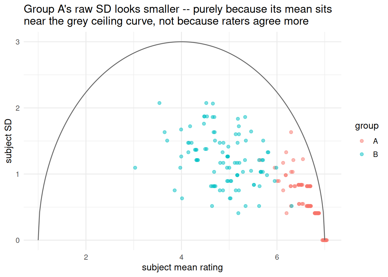
That imbalance --- not a difference in $\sigma$ --- shrinks Group A's raw SD.
When three-quarters of a subject's six ratings are forced into one bin by
`cut()`, the *discrete* variance across them is mechanically small, even though
the *continuous* latent draws behind them are as dispersed as Group B's
($\sigma=1$ for both). It is the same Bhatia--Davis mechanism from the
introduction, now visible subject by subject through `cut()`'s fixed boundaries
rather than through the population $\text{SD}_{\max}(\mu)$ curve.
The raw per-subject summary already shows the pattern that tempts a reader into
seeing a real disagreement gap:
```{r}
#| label: raw-summary
#| echo: true
#| message: false
#| warning: false
subj_summary <- df |>
group_by(subject, group) |>
summarise(mean_rating = mean(rating), sd_rating = sd(rating), .groups = "drop")
knitr::kable(
subj_summary |> group_by(group) |>
summarise(mean_of_means = round(mean(mean_rating), 2),
mean_of_sds = round(mean(sd_rating), 2)),
caption = "Raw per-subject summary by group -- true latent SD is IDENTICAL in both."
)
```
```{r}
#| label: scatter
#| echo: true
#| message: false
#| warning: false
#| fig-cap: "Subject-level mean vs. SD, with the theoretical ceiling overlaid."
ggplot(subj_summary, aes(mean_rating, sd_rating, color = group)) +
geom_jitter(width = 0.05, height = 0, alpha = 0.5) +
geom_line(data = data.frame(mean_rating = mu_grid, sd_rating = sd_max),
aes(mean_rating, sd_rating), color = "grey40", inherit.aes = FALSE) +
labs(x = "subject mean rating", y = "subject SD",
title = "Group A's raw SD looks smaller -- purely because its mean sits\nnear the grey ceiling curve, not because raters agree more") +
theme_minimal(base_size = 12)
```
Now fit both a Gaussian MELSM and the ordinal cumulative-probit MELSM to the
same data.
```{r}
#| label: fit-gaussian
#| echo: true
#| message: false
#| warning: false
#| cache: true
fit_gaussian <- brm(
bf(rating ~ group + (1 | subject), sigma ~ group),
data = df, family = gaussian(),
chains = 2, iter = 2000, warmup = 1000, cores = 2, seed = 1,
refresh = 0, silent = 2
)
```
```{r}
#| label: fit-ordinal
#| echo: true
#| message: false
#| warning: false
#| cache: true
fit_ordinal <- brm(
bf(rating_ord ~ group + (1 | subject), disc ~ 0 + group),
data = df, family = cumulative("probit"), init = 0,
prior = c(
prior(constant(0), class = "b", coef = "groupA", dpar = "disc"),
prior(normal(0, 1), class = "b", coef = "groupB", dpar = "disc")
),
chains = 2, iter = 2000, warmup = 1000, cores = 2, seed = 1,
refresh = 0, silent = 2
)
```
```{r}
#| label: compare-results
#| echo: true
#| message: false
#| warning: false
knitr::kable(round(fixef(fit_gaussian), 2), caption = "Gaussian MELSM fixed effects (sigma part is on the log-SD scale)")
knitr::kable(round(fixef(fit_ordinal), 2), caption = "Ordinal MELSM fixed effects (disc part is on the log scale: 0 = same latent SD as the reference group)")
```
On the raw scale Group A averages 6.64 with an SD of 0.58; Group B averages
4.89 with an SD of 1.22. The pooled correlation between subject mean and SD is
$-0.74$. That looks like a real, sizable disagreement gap, and the Gaussian
MELSM agrees: `sigma_groupB` of 0.68 on the log-SD scale puts Group B's SD at
**1.97 times** Group A's (95% CI: 1.82--2.14), nowhere near zero.
But there is no true difference. Both groups' raters were drawn with the same
$\sigma=1$ by construction; only the means differ. The ordinal model reads it
correctly: `disc_groupB` is $\gamma_B = -0.015$ on the log scale (95% CI:
$-0.171$ to $0.146$), so $\text{disc}_B = e^{-0.015} \approx 0.985$ --- a latent
SD of $\approx 1.015$ against the reference group's $1$, recovering the fact
that the two groups' dispersion is identical. The Gaussian model's "Group B
disagrees twice as much" is not a finding about the raters. It is the ceiling
effect from the previous section, wearing a regression coefficient.
### What about $R$ here?
$R$ is mean-independent by construction, so it should land where the ordinal
model does: no group difference. Compute it per subject, using the exact
finite-sample bound from the earlier callout ($n=6$ raters):
```{r}
#| label: r-measure
#| echo: true
#| message: false
#| warning: false
var_max_finite <- function(n, mu) {
c <- (mu - 1) / 6
a <- (n * c) %% 1
36 * (c * (1 - c) - (1 / n) * a * (1 - a))
}
subj_R <- df |>
group_by(subject, group) |>
summarise(mean_rating = mean(rating),
var_pop = mean((rating - mean(rating))^2), # population (1/n) convention
.groups = "drop") |>
mutate(var_max = var_max_finite(n_raters, mean_rating),
R = ifelse(var_max > 1e-8, var_pop / var_max, NA_real_))
knitr::kable(
subj_R |> group_by(group) |>
summarise(n_undefined = sum(is.na(R)), mean_R = round(mean(R, na.rm = TRUE), 3)),
caption = "Per-subject R, using each subject's own 6 ratings for both mean and variance."
)
```
This is worse than the raw SD comparison, not better. Group A's per-subject $R$
averages 0.63, Group B's 0.20 --- a larger apparent gap, and pointing the
*opposite* way from the ceiling artifact. Fourteen Group A subjects even have an
*undefined* $R$: all six raters picked 7, so observed variance and mechanical
ceiling are both zero at once. Has $R$ failed?
No. The guarantee --- $R\in[0,1]$ at every $\mu$, no forced link to the mean ---
is about the *population* quantity. Plug in a mean from only 6 raters and it
breaks, because the finite-sample bound in the denominator is itself estimated
from that same noisy mean, and it is far more sensitive near the ceiling than
mid-scale:
```{r}
#| label: r-diagnostic
#| echo: true
#| message: false
#| warning: false
knitr::kable(
subj_R |> group_by(group) |>
summarise(mean_var_pop = round(mean(var_pop), 3),
mean_var_max = round(mean(var_max, na.rm = TRUE), 3)),
caption = "The denominator (mean_var_max) is nearly 7x smaller for Group A -- not because Group A's true ceiling is that much tighter, but because a 6-rater sample mean near 7 makes the *estimated* ceiling collapse."
)
```
A Group A subject's six raters average near 7 because that is where their mean
sits --- but exactly *how* near is noisy, and the finite-sample bound shrinks
fast as the sample mean approaches the boundary. A modest observed variance over
an unluckily tiny denominator gives a large $R$, for no reason connected to real
disagreement. Swapping in the plain continuous bound shrinks the gap a great
deal --- 0.181 vs. 0.173 --- but each value still averages 100 noisy
single-subject estimates. Only pooling each group's full 600 ratings into one
mean and one variance removes the noise entirely:
```{r}
#| label: r-pooled
#| echo: true
#| message: false
#| warning: false
pooled <- df |> group_by(group) |>
summarise(mean_rating = mean(rating), var_pop = mean((rating - mean(rating))^2)) |>
mutate(var_max_cont = (mean_rating - 1) * (7 - mean_rating),
R_pooled = round(var_pop / var_max_cont, 3))
knitr::kable(pooled |> select(group, mean_rating, R_pooled),
caption = "R computed once per group, from all 600 ratings pooled.")
```
Pooled, $R$ is 0.22 for Group A and 0.21 for Group B --- essentially identical,
agreeing with the ordinal model's null finding. The lesson is not "avoid $R$."
It is that $R$, like $\varphi$, is only as good as the sample behind the mean and
variance you feed it. A hand-computed per-subject $R$ at 6 raters can
manufacture a *larger* spurious gap than raw SD, in the wrong direction. The
ordinal model never faces this, because it never forms a per-subject summary at
all. `disc_groupB` comes straight from the full, pooled 600-observation
likelihood per group --- the "pooled" calculation above done coherently, with a
proper posterior interval instead of an average of point estimates.
## Takeaways
::: {.callout-note}
## Summary
- On any bounded scale, the *maximum possible* variance is a function of the
mean --- the Bhatia--Davis inequality, $\text{Var}(X) \leq (\mu-a)(b-\mu)$.
Not a tendency to check for, a fact to design around.
- Dividing SD (or variance) by the mean does not remove the confound. The
mechanism is not proportional scaling; it is a ceiling that pinches at both
ends.
- A Gaussian location-scale model can estimate `sigma ~ x`, but inherits the
confound, because it has no boundary in it.
- Beta regression's precision $\varphi$ (and its bounded twin $R$) remove the
confound algebraically, at the cost of a continuous approximation to discrete
data. And $R$ is only as good as the sample behind it: with few raters per
subject, a hand-computed per-subject $R$ can manufacture a *larger* spurious
gap than raw SD, in the wrong direction --- and is undefined outright when
every rater picks the same endpoint of the scale, since then its numerator
and denominator vanish together.
- An ordinal cumulative-link mixed model puts the boundary where it belongs ---
estimated thresholds on a latent scale --- and is the cleanest way to ask "is
this dispersion difference real?" on Likert data, because it never needs a
per-unit summary statistic at all.
:::
## References
- Bhatia, R., and Davis, C. (2000). "A Better Bound on the Variance."
*American Mathematical Monthly* 107(4): 353--357.
- Bürkner, P.-C., and Vuorre, M. (2019). "Ordinal Regression Models in
Psychology: A Tutorial." *Advances in Methods and Practices in
Psychological Science* 2(1): 77--101.
- Cribari-Neto, F., and Zeileis, A. (2010). "Beta Regression in R." *Journal
of Statistical Software* 34(2): 1--24.
- Ellis, J. L. (2025). "The maximum variance of a finite dataset, given its
mean, minimum, and maximum."
[arXiv:2508.17525](https://arxiv.org/abs/2508.17525).
- Ferrari, S. L. P., and Cribari-Neto, F. (2004). "Beta Regression for
Modelling Rates and Proportions." *Journal of Applied Statistics* 31(7):
799--815.